|
PLUTO
|
Compute the curl of magnetic field. More...
#include "pluto.h"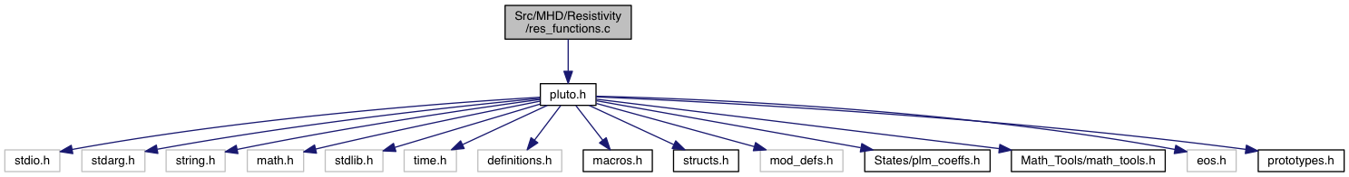
Go to the source code of this file.
Functions | |
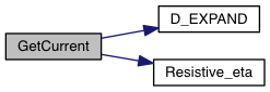
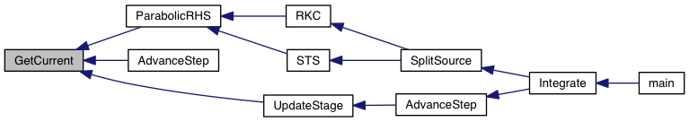
| void | GetCurrent (const Data *d, int dir, Grid *grid) |
Variables | |
| static double *** | eta [3] |
Compute the curl of magnetic field.
Compute the electric current (defined as J = curl(B)) for the induction and the total energy equations.
For constrained transport MHD, J has the same staggered location of the electric field and the three components (Jx, Jy, Jz) are placed at different locations inside the cell:
The same rule apply to the components of resistivity eta which are computed and stored inside this function.
For cell-centered MHD, the three components of J are computed during each sweep direction at cell interfaces, that is,
Although only the two transverse components of J are actually needed during the update step, we compute also the normal component since the resistivity coefficients eta may depend on the total current.
For a compact implementation, we note that the curl of a vector in the three system of coordinates normally adopted may be written as
![\[ \begin{array}{lcl} \left(\nabla\times\vec{B}\right)_{x_1} &=& \DS \frac{1}{d_{23}}\pd{}{x_2}(a_{23}B_{x_3}) - \frac{1}{d_{32}}\pd{B_{x_2}}{x_3} \\ \noalign{\bigskip} \left(\nabla\times\vec{B}\right)_{x_2} &=& \DS \frac{1}{d_{31}}\pd{B_{x_1}}{x_3} - \frac{1}{d_{13}}\pd{}{x_1}(a_{13}B_{x_3}) \\ \noalign{\bigskip} \left(\nabla\times\vec{B}\right)_{x_3} &=& \DS \frac{1}{d_{12}}\pd{}{x_1}(a_{12}B_{x_2}) - \frac{1}{d_{21}}\pd{B_{x_1}}{x_2} \end{array} \]](form_99.png)
where the coefficients  and
and  except:
![\[ \begin{array}{lll} d_{nm} = 1; & \quad a_{nm} = 1; & \qquad ({\rm Cartesian}) \\ \noalign{\medskip} d_{13} = r\,,\qquad & d_{32} = d_{31} = \infty; \quad a_{13} = r; & \qquad ({\rm Cylindrical}) \\ \noalign{\medskip} d_{23} = d_{12} = d_{21} = r; & \quad a_{12} = r; & \qquad ({\rm Polar}) \\ \noalign{\medskip} d_{23} = d_{32} = d_{31} = r\sin\theta \,,\qquad d_{13} = d_{12} = d_{21} = r; & \quad a_{23} = \sin\theta\,,\qquad a_{13} = a_{12} = r; & \qquad ({\rm Spherical}) \end{array} \]](form_102.png)
In the actual implementation we use  .
.
Definition in file res_functions.c.
Compute the curl of magnetic field for constrained transport MHD or cell-centered MHD.
| [in,out] | d | pointer to the PLUTO data structure |
| [in] | dir | sweep direction (useless for constrained transport MHD) |
| [in] | grid | pointer to an array of Grid structures |
4b. For cell-centered MHD, we compute the three components of
Definition at line 97 of file res_functions.c.
|
static |
Definition at line 94 of file res_functions.c.
 1.8.10
