|
PLUTO
|
Rayleigh-Taylor instability setup for hydro or MHD. More...
#include "pluto.h"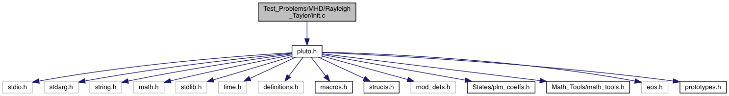
Go to the source code of this file.
Functions | |
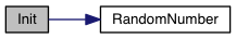
| void | Init (double *v, double x1, double x2, double x3) |
| void | Analysis (const Data *d, Grid *grid) |
| void | UserDefBoundary (const Data *d, RBox *box, int side, Grid *grid) |
Rayleigh-Taylor instability setup for hydro or MHD.
Sets the initial condition for a Rayleigh-Taylor instability problem in 2 or 3 dimensions. The initial condition consists of an interface separating two fluids with different densities in hydrostatic balance:
![\[ \rho(y) = \left\{\begin{array}{ll} 1 & \quad{\rm for} \quad y \le 0 \\ \noalign{\medskip} \eta & \quad{\rm for} \quad y > 0 \end{array}\right. \,,\qquad p = p_0 + \rho y g \]](form_351.png)
where  is the density of the fluid on top,
 g is the (constant) gravity pointing in the negative y direction. The value of the pressure at the interface (p0) is chosen in such a way that the sound speed in the light fluid is 1. Likewise, density is normalized to the value in the light fluid. The horizontal extent of the computational domain defines the unit length: Lx=1.
For magnetized setups, the magnetic field is purely horizontal:
![\[ \vec{B} = \chi B_c\hvec{i} \,,\qquad B_c \equiv \sqrt{(\rho_{\rm hi} - \rho_{\rm lo})L|g|}\quad \to\quad \sqrt{(\eta - 1.0)|g|} \]](form_353.png)
where Bc is the critical magnetic field above which perturbations parallel to the magnetic field are suppressed (see Boyd & Sanderson, page 99) while the value of  is user-supplied (note that a factor
  needs to be incorporated when initializing
 B in code units).
The system is destabilized by perturbing the vertical velocity in proximity of the interface using a single mode (in 2D) or a Gaussian perturbation (in 3D). Aleternatively, a random perturbation can be used by setting USE_RANDOM_PERTURBATION to YES in your definitions.h. The runtime parameters that are read from pluto.ini are
g_inputParam[ETA]: sets the density of the upper fluid;g_inputParam[GRAV]: sets gravity (must be < 0);g_inputParam[CHI]: sets the magnetic field strength in unit of the critical magnetic field Bc;p0 by a factor q^2 is equivalent to increase gravity of the same factor and decrease velocity and time by a factor q.The Rayleigh-Taylor setup has been tested with the following configurations:
| Conf. | PHYSICS | GEOMETRY | DIM | T. STEP. | INTERP. | divB | Notes |
|---|---|---|---|---|---|---|---|
| #01 | HD | CARTESIAN | 2 | HANCOCK | LINEAR | - | - |
| #02 | HD | CARTESIAN | 2 | RK3 | MP5_FD | - | - |
| #03 | HD | CARTESIAN | 2 | RK3 | PARABOLIC | - | - |
| #04 | HD | CARTESIAN | 2 | RK2 | LINEAR | - | (*) |
| #05 | MHD | CARTESIAN | 2 | HANCOCK | LINEAR | CT | - |
| #06 | MHD | CARTESIAN | 2 | RK3 | MP5_FD | GLM | - |
| #07 | MHD | CARTESIAN | 2 | RK3 | PARABOLIC | CT | - |
| #08 | MHD | CARTESIAN | 2 | ChTr | PARABOLIC | GLM | (*) |
| #09 | MHD | CARTESIAN | 3 | RK2 | LINEAR | GLM | - |
| #10 | MHD | CARTESIAN | 3 | HANCOCK | LINEAR | GLM | [Mig12](*) |
(*) Setups for AMR-Chombo

References:
Definition in file init.c.
| void Init | ( | double * | v, |
| double | x1, | ||
| double | x2, | ||
| double | x3 | ||
| ) |
The Init() function can be used to assign initial conditions as as a function of spatial position.
| [out] | v | a pointer to a vector of primitive variables |
| [in] | x1 | coordinate point in the 1st dimension |
| [in] | x2 | coordinate point in the 2nd dimension |
| [in] | x3 | coordinate point in the 3rdt dimension |
The meaning of x1, x2 and x3 depends on the geometry:
![\[ \begin{array}{cccl} x_1 & x_2 & x_3 & \mathrm{Geometry} \\ \noalign{\medskip} \hline x & y & z & \mathrm{Cartesian} \\ \noalign{\medskip} R & z & - & \mathrm{cylindrical} \\ \noalign{\medskip} R & \phi & z & \mathrm{polar} \\ \noalign{\medskip} r & \theta & \phi & \mathrm{spherical} \end{array} \]](form_173.png)
Variable names are accessed by means of an index v[nv], where nv = RHO is density, nv = PRS is pressure, nv = (VX1, VX2, VX3) are the three components of velocity, and so forth.
Definition at line 86 of file init.c.
Assign user-defined boundary conditions.
| [in,out] | d | pointer to the PLUTO data structure containing cell-centered primitive quantities (d->Vc) and staggered magnetic fields (d->Vs, when used) to be filled. |
| [in] | box | pointer to a RBox structure containing the lower and upper indices of the ghost zone-centers/nodes or edges at which data values should be assigned. |
| [in] | side | specifies the boundary side where ghost zones need to be filled. It can assume the following pre-definite values: X1_BEG, X1_END, X2_BEG, X2_END, X3_BEG, X3_END. The special value side == 0 is used to control a region inside the computational domain. |
| [in] | grid | pointer to an array of Grid structures. |
Assign user-defined boundary conditions in the lower boundary ghost zones. The profile is top-hat:
![\[ V_{ij} = \left\{\begin{array}{ll} V_{\rm jet} & \quad\mathrm{for}\quad r_i < 1 \\ \noalign{\medskip} \mathrm{Reflect}(V) & \quad\mathrm{otherwise} \end{array}\right. \]](form_235.png)
where  and
and M is the flow Mach number (the unit velocity is the jet sound speed, so  ).
).
Assign user-defined boundary conditions:
x < 1/6 and reflective boundary otherwise. we use fixed (post-shock) values. Unperturbed values otherwise.
Assign user-defined boundary conditions at inner and outer radial boundaries. Reflective conditions are applied except for the azimuthal velocity which is fixed.
Assign user-defined boundary conditions.
| [in/out] | d pointer to the PLUTO data structure containing cell-centered primitive quantities (d->Vc) and staggered magnetic fields (d->Vs, when used) to be filled. | |
| [in] | box | pointer to a RBox structure containing the lower and upper indices of the ghost zone-centers/nodes or edges at which data values should be assigned. |
| [in] | side | specifies on which side boundary conditions need to be assigned. side can assume the following pre-definite values: X1_BEG, X1_END, X2_BEG, X2_END, X3_BEG, X3_END. The special value side == 0 is used to control a region inside the computational domain. |
| [in] | grid | pointer to an array of Grid structures. |
Set the injection boundary condition at the lower z-boundary (X2-beg must be set to userdef in pluto.ini). For  we set constant input values (given by the GetJetValues() function while for $ R > 1 $ the solution has equatorial symmetry with respect to the
 z=0 plane. To avoid numerical problems with a "top-hat" discontinuous jump, we smoothly merge the inlet and reflected value using a profile function Profile().
 1.8.10
