|
PLUTO
|
Axisymmetric jet propagation. More...
#include "pluto.h"
Go to the source code of this file.
Functions | |
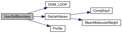
| void | GetJetValues (double, double *) |
| static double | Profile (double, double) |
| void | Init (double *v, double x1, double x2, double x3) |
| void | Analysis (const Data *d, Grid *grid) |
| void | UserDefBoundary (const Data *d, RBox *box, int side, Grid *grid) |
Variables | |
| static double | a = 0.8 |
| static double | Ta |
| static double | pa |
| static double | mua |
Axisymmetric jet propagation.
Description.
The jet problem is set up in axisymmetric cylindrical coordinates  . We label ambient and jet values with the suffix "a" and "j", respectively. The ambient medium is at rest and is characterized by uniform density and pressure,
  and
and  . The beam enters from the lower-z boundary from a circular nozzle of radius
  and carries a constant poloidal field
  and a (radially-varying) toroidal component
  . Flow variables are prescribed as
![\[ \left\{\begin{array}{lcl} \rho(R) &=& \rho_j \\ \noalign{\medskip} v_z(R) &=& v_j \\ \noalign{\medskip} B_\phi(R) &=& \DS \left\{\begin{array}{ll} -B_m R/a & \quad{\rm for}\quad R<a \\ \noalign{\medskip} -B_m a/R & \quad{\rm for}\quad R>a \end{array}\right. \\ \noalign{\medskip} B_z(R) &=& B_{z0}\quad\mathrm{(const)} \end{array}\right. \]](form_333.png)
Here a is the magnetization radius while  . These profiles are similar to the ones used by Tesileanu et al. (2008). The pressure distribution is found by solving the radial momentum balance between thermal, centrifugal and magnetic forces:
![\[ \frac{dp}{dR} = \frac{\rho v_\phi^2}{R} - \frac{1}{2}\left[\frac{1}{R^2}\frac{d(R^2B^2_\phi)}{dR} +\frac{dB_z^2}{dR}\right] \]](form_335.png)
Neglecting rotation and assuming Bz to be constant the solution of radial momentum balance becomes
![\[ p(R) = p_a + B_m^2\left[1-\min\left(\frac{R^2}{a^2},1\right)\right] \]](form_336.png)
and the jet on-axis pressure increases for increasing toroidal field:
![\[ p(R=0) \equiv p_j = p_a + B_m^2 \]](form_337.png)
where  is the ambient pressure.
Normalization.
Since the MHD equations are scale-invariant we have the freedom to specify a reference length, density and velocity. Here we choose
 ;
; ;
; (from which it follows
  ).
).UNIT_VELOCITY). In this case, the ambient pressure is computed from the ambient temperature Ta = 2500 K .In this way the number of parameters is reduced to 4:
g_inputParam[ETA]: density contrast 
g_inputParam[JET_VEL]: Jet velocity  . This is also the Mach number of the beam with respect to the ambient in the adiabatic setup;
g_inpurParam[SIGMA_Z]: poloidal magnetization;g_inpurParam[SIGMA_PHI]: toroidal magnetization; Magnetization are defined as follows:
![\[ \left\{\begin{array}{ll} \sigma_z &= \DS \frac{B_z^2}{2p_a} \\ \noalign{\medskip} \sigma_\phi &= \DS \frac{<B_\phi^2>}{2p_a} \end{array}\right. \qquad\Longrightarrow\qquad \left\{\begin{array}{ll} B_z^2 &= \DS 2\sigma_zp_a \\ \noalign{\medskip} B_m^2 &= \DS \frac{2\sigma_\phi}{a^2(1/2-2\log a)}p_a \end{array}\right. \]](form_345.png)
 is simply found as
![\[ <B^2_\phi> = \frac{\int_0^1 B^2_\phi R\,dR}{\int_0^1 R\,dR} = B_m^2a^2\left(\frac{1}{2} - 2\log a\right) \]](form_347.png)
The following MAPLE code can be used to verify the solution:
When cooling is enabled, two additional parameters controlling the amplitude and frequency of perturbation can be used:
g_inputParam[PERT_AMPLITUDE]: perturbation amplitude (in units of jet velocity);g_inputParam[PERT_PERIOD]: perturbation period (in years).The jet problem has been tested using a variety of configurations, namely:
| Conf. | GEOMETRY | DIM | T. STEPPING | RECONSTRUCTION | divB | EOS | COOLING |
|---|---|---|---|---|---|---|---|
| #01 | CYLINDRICAL | 2 | RK2 | LINEAR | CT | IDEAL | NO |
| #02 | CYLINDRICAL | 2 | HANCOCK | LINEAR | CT | IDEAL | NO |
| #03 | CYLINDRICAL | 2 | ChTr | PARABOLIC | CT | IDEAL | NO |
| #04 | CYLINDRICAL | 2.5 | RK2 | LINEAR | NONE | IDEAL | NO |
| #05 | CYLINDRICAL | 2.5 | RK2 | LINEAR | CT | IDEAL | NO |
| #06 | CYLINDRICAL | 2.5 | RK2 | LINEAR | CT | PVTE_LAW | NO |
| #07 | CYLINDRICAL | 2.5 | ChTr | PARABOLIC | NONE | IDEAL | SNEq |
| #08 | CYLINDRICAL | 2.5 | ChTr | PARABOLIC | NONE | IDEAL | MINEq |
| #09 | CYLINDRICAL | 2.5 | ChTr | PARABOLIC | NONE | IDEAL | H2_COOL |
Here 2.5 is a short-cut for to 2 dimensions and 3 components.
The following image show the (log) density map at the end of simulation for setup #01.

References
Definition in file init.c.
| void GetJetValues | ( | double | R, |
| double * | vj | ||
| ) |
Define jet value as functions of the (cylindrical) radial coordinate. For a periodic jet configuration, density and verical velocity smoothly join the ambient values. This has no effect on equilibrium as long as rotation profile depends on the chosen density profile.
Definition at line 264 of file init.c.
| void Init | ( | double * | v, |
| double | x1, | ||
| double | x2, | ||
| double | x3 | ||
| ) |
The Init() function can be used to assign initial conditions as as a function of spatial position.
| [out] | v | a pointer to a vector of primitive variables |
| [in] | x1 | coordinate point in the 1st dimension |
| [in] | x2 | coordinate point in the 2nd dimension |
| [in] | x3 | coordinate point in the 3rdt dimension |
The meaning of x1, x2 and x3 depends on the geometry:
![\[ \begin{array}{cccl} x_1 & x_2 & x_3 & \mathrm{Geometry} \\ \noalign{\medskip} \hline x & y & z & \mathrm{Cartesian} \\ \noalign{\medskip} R & z & - & \mathrm{cylindrical} \\ \noalign{\medskip} R & \phi & z & \mathrm{polar} \\ \noalign{\medskip} r & \theta & \phi & \mathrm{spherical} \end{array} \]](form_173.png)
Variable names are accessed by means of an index v[nv], where nv = RHO is density, nv = PRS is pressure, nv = (VX1, VX2, VX3) are the three components of velocity, and so forth.
Definition at line 139 of file init.c.
|
static |
Set the injection boundary condition at the lower z-boundary (X2-beg must be set to userdef in pluto.ini). For  we set constant input values (given by the GetJetValues() function while for $ R > 1 $ the solution has equatorial symmetry with respect to the
 z=0 plane. To avoid numerical problems with a "top-hat" discontinuous jump, we smoothly merge the inlet and reflected value using a profile function Profile().
Definition at line 196 of file init.c.
 1.8.10