PLUTO
pyPLUTO.pyPLUTO.Image Class Reference
Inheritance diagram for pyPLUTO.pyPLUTO.Image:
Collaboration diagram for pyPLUTO.pyPLUTO.Image:

Public Member Functions

def pldisplay (self, D, var, kwargs)
 
def multi_disp (self, args, kwargs)
 
def oplotbox
 
def field_interp (self, var1, var2, x, y, dx, dy, xp, yp)
 
def field_line (self, var1, var2, x, y, dx, dy, x0, y0)
 
def myfieldlines (self, Data, x0arr, y0arr, stream=False, kwargs)
 
def getSphData (self, Data, w_dir=None, datatype=None, kwargs)
 
def getPolarData
 
def pltSphData (self, Data, w_dir=None, datatype=None, kwargs)
 

Detailed Description

This Class has all the routines for the imaging the data
and plotting various contours and fieldlines on these images.
CALLED AFTER pyPLUTO.pload object is defined

Definition at line 1247 of file pyPLUTO.py.

Member Function Documentation

def pyPLUTO.pyPLUTO.Image.field_interp (   self,
  var1,
  var2,
  x,
  y,
  dx,
  dy,
  xp,
  yp 
)
This method interpolates value of vector fields (var1 and var2) on field points (xp and yp).
The field points are obtained from the method field_line.

**Inputs:**

  var1 -- 2D Vector field in X direction\n
  var2 -- 2D Vector field in Y direction\n
  x -- 1D X array\n
  y -- 1D Y array\n
  dx -- 1D grid spacing array in X direction\n
  dy -- 1D grid spacing array in Y direction\n
  xp -- field point in X direction\n
  yp -- field point in Y direction\n
  
**Outputs:**

  A list with 2 elements where the first element corresponds to the interpolate field 
  point in 'x' direction and the second element is the field point in 'y' direction.  

Definition at line 1410 of file pyPLUTO.py.

1410  def field_interp(self,var1,var2,x,y,dx,dy,xp,yp):
1411  """ This method interpolates value of vector fields (var1 and var2) on field points (xp and yp).
1412  The field points are obtained from the method field_line.
1413 
1414  **Inputs:**
1415 
1416  var1 -- 2D Vector field in X direction\n
1417  var2 -- 2D Vector field in Y direction\n
1418  x -- 1D X array\n
1419  y -- 1D Y array\n
1420  dx -- 1D grid spacing array in X direction\n
1421  dy -- 1D grid spacing array in Y direction\n
1422  xp -- field point in X direction\n
1423  yp -- field point in Y direction\n
1424 
1425  **Outputs:**
1426 
1427  A list with 2 elements where the first element corresponds to the interpolate field
1428  point in 'x' direction and the second element is the field point in 'y' direction.
1429 
1430  """
1431  q=[]
1432  U = var1
1433  V = var2
1434  i0 = np.abs(xp-x).argmin()
1435  j0 = np.abs(yp-y).argmin()
1436  scrhUx = np.interp(xp,x,U[:,j0])
1437  scrhUy = np.interp(yp,y,U[i0,:])
1438  q.append(scrhUx + scrhUy - U[i0,j0])
1439  scrhVx = np.interp(xp,x,V[:,j0])
1440  scrhVy = np.interp(yp,y,V[i0,:])
1441  q.append(scrhVx + scrhVy - V[i0,j0])
1442  return q
1443 
def field_interp(self, var1, var2, x, y, dx, dy, xp, yp)
Definition: pyPLUTO.py:1410

Here is the caller graph for this function:

def pyPLUTO.pyPLUTO.Image.field_line (   self,
  var1,
  var2,
  x,
  y,
  dx,
  dy,
  x0,
  y0 
)
This method is used to obtain field lines (same as fieldline.pro in PLUTO IDL tools).
    
**Inputs:**
    
  var1 -- 2D Vector field in X direction\n
  var2 -- 2D Vector field in Y direction\n
  x -- 1D X array\n
  y -- 1D Y array\n
  dx -- 1D grid spacing array in X direction\n
  dy -- 1D grid spacing array in Y direction\n
  x0 -- foot point of the field line in X direction\n
  y0 -- foot point of the field line in Y direction\n
  
**Outputs:**
    
  This routine returns a dictionary with keys - \n
  qx -- list of the field points along the 'x' direction.
  qy -- list of the field points along the 'y' direction.
  
**Usage:**
  
  See the myfieldlines routine for the same.          

Definition at line 1444 of file pyPLUTO.py.

1444  def field_line(self,var1,var2,x,y,dx,dy,x0,y0):
1445  """ This method is used to obtain field lines (same as fieldline.pro in PLUTO IDL tools).
1446 
1447  **Inputs:**
1448 
1449  var1 -- 2D Vector field in X direction\n
1450  var2 -- 2D Vector field in Y direction\n
1451  x -- 1D X array\n
1452  y -- 1D Y array\n
1453  dx -- 1D grid spacing array in X direction\n
1454  dy -- 1D grid spacing array in Y direction\n
1455  x0 -- foot point of the field line in X direction\n
1456  y0 -- foot point of the field line in Y direction\n
1457 
1458  **Outputs:**
1459 
1460  This routine returns a dictionary with keys - \n
1461  qx -- list of the field points along the 'x' direction.
1462  qy -- list of the field points along the 'y' direction.
1463 
1464  **Usage:**
1465 
1466  See the myfieldlines routine for the same.
1467  """
1468  xbeg = x[0] - 0.5*dx[0]
1469  xend = x[-1] + 0.5*dx[-1]
1470 
1471  ybeg = y[0] - 0.5*dy[0]
1472  yend = y[-1] + 0.5*dy[-1]
1473 
1474  inside_domain = x0 > xbeg and x0 < xend and y0 > ybeg and y0 < yend
1475 
1476  MAX_STEPS = 5000
1477  xln_fwd = [x0]
1478  yln_fwd = [y0]
1479  xln_bck = [x0]
1480  yln_bck = [y0]
1481  rhs = []
1482  k = 0
1483 
1484  while inside_domain == True:
1485  R1 = self.field_interp(var1,var2,x,y,dx,dy,xln_fwd[k],yln_fwd[k])
1486  dl = 0.5*np.max(np.concatenate((dx,dy)))/(np.sqrt(R1[0]*R1[0] + R1[1]*R1[1] + 1.e-14))
1487  xscrh = xln_fwd[k] + 0.5*dl*R1[0]
1488  yscrh = yln_fwd[k] + 0.5*dl*R1[1]
1489 
1490  R2 = self.field_interp(var1,var2,x,y,dx,dy,xln_fwd[k],yln_fwd[k])
1491 
1492  xln_one = xln_fwd[k] + dl*R2[0]
1493  yln_one = yln_fwd[k] + dl*R2[1]
1494 
1495  xln_fwd.append(xln_one)
1496  yln_fwd.append(yln_one)
1497  inside_domain = xln_one > xbeg and xln_one < xend and yln_one > ybeg and yln_one < yend
1498  inside_domain = inside_domain and (k < MAX_STEPS-3)
1499  k = k + 1
1500 
1501 
1502  k_fwd = k
1503  qx = np.asarray(xln_fwd[0:k_fwd])
1504  qy = np.asarray(yln_fwd[0:k_fwd])
1505  flines={'qx':qx,'qy':qy}
1506 
1507  return flines
1508 
1509 
def field_line(self, var1, var2, x, y, dx, dy, x0, y0)
Definition: pyPLUTO.py:1444
def field_interp(self, var1, var2, x, y, dx, dy, xp, yp)
Definition: pyPLUTO.py:1410

Here is the call graph for this function:

Here is the caller graph for this function:

def pyPLUTO.pyPLUTO.Image.getPolarData (   self,
  Data,
  ang_coord,
  rphi = False 
)
To get the Cartesian Co-ordinates from Polar.

**Inputs:**

  Data -- pyPLUTO pload Object\n
  ang_coord -- The Angular co-ordinate (theta or Phi)
 
*Optional Keywords:*

  rphi -- Default value FALSE is for R-THETA data, 
  Set TRUE for R-PHI data.\n

**Outputs**:

  2D Arrays of X, Y from the Radius and Angular co-ordinates.\n
  They are used in pcolormesh in the Image.pldisplay functions.

Definition at line 1642 of file pyPLUTO.py.
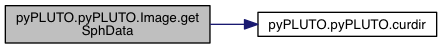
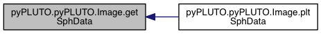
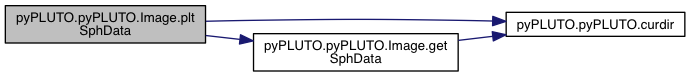
1642  def getPolarData(self, Data, ang_coord, rphi=False):
1643  """To get the Cartesian Co-ordinates from Polar.
1644 
1645  **Inputs:**
1646 
1647  Data -- pyPLUTO pload Object\n
1648  ang_coord -- The Angular co-ordinate (theta or Phi)
1649 
1650  *Optional Keywords:*
1651 
1652  rphi -- Default value FALSE is for R-THETA data,
1653  Set TRUE for R-PHI data.\n
1654 
1655  **Outputs**:
1656 
1657  2D Arrays of X, Y from the Radius and Angular co-ordinates.\n
1658  They are used in pcolormesh in the Image.pldisplay functions.
1659  """
1660  D = Data
1661  if ang_coord is D.x2:
1662  x2r = D.x2r
1663  elif ang_coord is D.x3:
1664  x2r = D.x3r
1665  else:
1666  print "Angular co-ordinate must be given"
1667 
1668  rcos = np.outer(np.cos(x2r), D.x1r)
1669  rsin = np.outer(np.sin(x2r), D.x1r)
1670 
1671  if rphi:
1672  xx = rcos
1673  yy = rsin
1674  else:
1675  xx = rsin
1676  yy = rcos
1677 
1678  return xx, yy
1679 

Here is the caller graph for this function:

def pyPLUTO.pyPLUTO.Image.getSphData (   self,
  Data,
  w_dir = None,
  datatype = None,
  kwargs 
)
This method transforms the vector and scalar  fields from Spherical co-ordinates to Cylindrical.

**Inputs**:

  Data -- pyPLUTO.pload object\n
  w_dir -- /path/to/the/working/directory/\n
  datatype -- If the data is of 'float' type then datatype = 'float' else by default the datatype is set to 'double'.

*Optional Keywords*:

      rphi -- [Default] is set to False implies that the r-theta plane is transformed. If set True then the r-phi plane is transformed.\n
  x2cut -- Applicable for 3D data and it determines the co-ordinate of the x2 plane while r-phi is set to True.\n
  x3cut -- Applicable for 3D data and it determines the co-ordinate of the x3 plane while r-phi is set to False.

Definition at line 1562 of file pyPLUTO.py.

1562  def getSphData(self,Data,w_dir=None,datatype=None,**kwargs):
1563  """This method transforms the vector and scalar fields from Spherical co-ordinates to Cylindrical.
1564 
1565  **Inputs**:
1566 
1567  Data -- pyPLUTO.pload object\n
1568  w_dir -- /path/to/the/working/directory/\n
1569  datatype -- If the data is of 'float' type then datatype = 'float' else by default the datatype is set to 'double'.
1570 
1571  *Optional Keywords*:
1572 
1573  rphi -- [Default] is set to False implies that the r-theta plane is transformed. If set True then the r-phi plane is transformed.\n
1574  x2cut -- Applicable for 3D data and it determines the co-ordinate of the x2 plane while r-phi is set to True.\n
1575  x3cut -- Applicable for 3D data and it determines the co-ordinate of the x3 plane while r-phi is set to False.
1576 
1577  """
1578 
1579  Tool = Tools()
1580  key_value_pairs = []
1581  allvars = []
1582  if w_dir is None: w_dir = curdir()
1583  for v in Data.vars:
1584  allvars.append(v)
1585 
1586  if kwargs.get('rphi',False)==True:
1587  R,TH = np.meshgrid(Data.x1,Data.x3)
1588  if Data.n3 != 1:
1589  for variable in allvars:
1590  key_value_pairs.append([variable,getattr(Data,variable)[:,kwargs.get('x2cut',0),:].T])
1591 
1592  SphData = dict(key_value_pairs)
1593  if ('bx1' in allvars) or ('bx2' in allvars):
1594  (SphData['b1c'],SphData['b3c']) = Tool.RTh2Cyl(R,TH,SphData.get('bx1'),SphData.get('bx3'))
1595  allvars.append('b1c')
1596  allvars.append('b3c')
1597  if ('vx1' in allvars) or ('vx2' in allvars):
1598  (SphData['v1c'],SphData['v3c']) = Tool.RTh2Cyl(R,TH,SphData.get('vx1'),SphData.get('vx3'))
1599  allvars.append('v1c')
1600  allvars.append('v3c')
1601  else:
1602  print "No x3 plane for 2D data"
1603  else:
1604  R,TH = np.meshgrid(Data.x1,Data.x2)
1605  if Data.n3 != 1:
1606  for variable in allvars:
1607  key_value_pairs.append([variable,getattr(Data,variable)[:,:,kwargs.get('x3cut',0)].T])
1608  SphData = dict(key_value_pairs)
1609  if ('bx1' in allvars) or ('bx2' in allvars):
1610  (SphData['b1c'],SphData['b2c']) = Tool.RTh2Cyl(R,TH,SphData.get('bx1'),SphData.get('bx2'))
1611  allvars.append('b1c')
1612  allvars.append('b2c')
1613  if ('vx1' in allvars) or ('vx2' in allvars):
1614  (SphData['v1c'],SphData['v2c']) = Tool.RTh2Cyl(R,TH,SphData.get('vx1'),SphData.get('vx2'))
1615  allvars.append('v1c')
1616  allvars.append('v2c')
1617  else:
1618  for variable in allvars:
1619  key_value_pairs.append([variable,getattr(Data,variable)[:,:].T])
1620  SphData = dict(key_value_pairs)
1621  if ('bx1' in allvars) or ('bx2' in allvars):
1622  (SphData['b1c'],SphData['b2c']) = Tool.RTh2Cyl(R,TH,SphData.get('bx1'),SphData.get('bx2'))
1623  allvars.append('b1c')
1624  allvars.append('b2c')
1625  if ('vx1' in allvars) or ('vx2' in allvars):
1626  (SphData['v1c'],SphData['v2c']) = Tool.RTh2Cyl(R,TH,SphData.get('vx1'),SphData.get('vx2'))
1627  allvars.append('v1c')
1628  allvars.append('v2c')
1629 
1630  for variable in allvars:
1631  if kwargs.get('rphi',False)==True:
1632  R,Z,SphData[variable]= Tool.sph2cyl(Data,SphData.get(variable),rphi=True,theta0=Data.x2[kwargs.get('x2cut',0)])
1633  else:
1634  if Data.n3 != 1:
1635  R,Z,SphData[variable] = Tool.sph2cyl(Data,SphData.get(variable),rphi=False)
1636  else:
1637  R,Z,SphData[variable] = Tool.sph2cyl(Data,SphData.get(variable),rphi=False)
1638 
1639  return R,Z,SphData
1640 
1641 
def getSphData(self, Data, w_dir=None, datatype=None, kwargs)
Definition: pyPLUTO.py:1562
def curdir()
Definition: pyPLUTO.py:19

Here is the call graph for this function:

Here is the caller graph for this function:

def pyPLUTO.pyPLUTO.Image.multi_disp (   self,
  args,
  kwargs 
)

Definition at line 1314 of file pyPLUTO.py.

1314  def multi_disp(self,*args,**kwargs):
1315  mvar = []
1316  for arg in args:
1317  mvar.append(arg.T)
1318 
1319  xmin = np.min(kwargs.get('x1'))
1320  xmax = np.max(kwargs.get('x1'))
1321  ymin = np.min(kwargs.get('x2'))
1322  ymax = np.max(kwargs.get('x2'))
1323  mfig = figure(kwargs.get('fignum',1),figsize=kwargs.get('figsize',[10,10]))
1324  Ncols = kwargs.get('Ncols')
1325  Nrows = len(args)/Ncols
1326  mprod = Nrows*Ncols
1327  dictcbar=kwargs.get('cbar',(False,'','each'))
1328 
1329  for j in range(mprod):
1330  mfig.add_subplot(Nrows,Ncols,j+1)
1331  pcolormesh(kwargs.get('x1'),kwargs.get('x2'), mvar[j])
1332  axis([xmin,xmax,ymin,ymax])
1333  gca().set_aspect('equal')
1334 
1335  xlabel(kwargs.get('label1',mprod*['Xlabel'])[j])
1336  ylabel(kwargs.get('label2',mprod*['Ylabel'])[j])
1337  title(kwargs.get('title',mprod*['Title'])[j])
1338  if (dictcbar[0] == True) and (dictcbar[2] =='each'):
1339  colorbar(orientation=kwargs.get('cbar')[1])
1340  if dictcbar[0] == True and dictcbar[2]=='last':
1341  if (j == np.max(range(mprod))):colorbar(orientation=kwargs.get('cbar')[1])
1342 
string title
Definition: jet.py:14
def multi_disp(self, args, kwargs)
Definition: pyPLUTO.py:1314

Here is the call graph for this function:

def pyPLUTO.pyPLUTO.Image.myfieldlines (   self,
  Data,
  x0arr,
  y0arr,
  stream = False,
  kwargs 
)
This method overplots the magnetic field lines at the footpoints given by (x0arr[i],y0arr[i]).

**Inputs:**

  Data -- pyPLUTO.pload object\n
  x0arr -- array of x co-ordinates of the footpoints\n
  y0arr -- array of y co-ordinates of the footpoints\n
  stream -- keyword for two different ways of calculating the field lines.\n
  True -- plots contours of rAphi (needs to store vector potential)\n
  False -- plots the fieldlines obtained from the field_line routine. (Default option)
  
*Optional Keywords:*

  colors -- A list of matplotlib colors to represent the lines. The length of this list should be same as that of x0arr.\n
  lw -- Integer value that determines the linewidth of each line.\n
  ls -- Determines the linestyle of each line.

**Usage:**
  
  Assume that the magnetic field is a given as **B** = B0$\hat{y}$. 
  Then to show this field lines we have to define the x and y arrays of field foot points.\n 
  
  ``x0arr = linspace(0.0,10.0,20)``\n
  ``y0arr = linspace(0.0,0.0,20)``\n
  ``import pyPLUTO as pp``\n
  ``D = pp.pload(45)``\n
  ``I = pp.Image()``\n
  ``I.myfieldlines(D,x0arr,y0arr,colors='k',ls='--',lw=1.0)``

Definition at line 1510 of file pyPLUTO.py.

1510  def myfieldlines(self,Data,x0arr,y0arr,stream=False,**kwargs):
1511  """ This method overplots the magnetic field lines at the footpoints given by (x0arr[i],y0arr[i]).
1512 
1513  **Inputs:**
1514 
1515  Data -- pyPLUTO.pload object\n
1516  x0arr -- array of x co-ordinates of the footpoints\n
1517  y0arr -- array of y co-ordinates of the footpoints\n
1518  stream -- keyword for two different ways of calculating the field lines.\n
1519  True -- plots contours of rAphi (needs to store vector potential)\n
1520  False -- plots the fieldlines obtained from the field_line routine. (Default option)
1521 
1522  *Optional Keywords:*
1523 
1524  colors -- A list of matplotlib colors to represent the lines. The length of this list should be same as that of x0arr.\n
1525  lw -- Integer value that determines the linewidth of each line.\n
1526  ls -- Determines the linestyle of each line.
1527 
1528  **Usage:**
1529 
1530  Assume that the magnetic field is a given as **B** = B0$\hat{y}$.
1531  Then to show this field lines we have to define the x and y arrays of field foot points.\n
1532 
1533  ``x0arr = linspace(0.0,10.0,20)``\n
1534  ``y0arr = linspace(0.0,0.0,20)``\n
1535  ``import pyPLUTO as pp``\n
1536  ``D = pp.pload(45)``\n
1537  ``I = pp.Image()``\n
1538  ``I.myfieldlines(D,x0arr,y0arr,colors='k',ls='--',lw=1.0)``
1539  """
1540 
1541  if len(x0arr) != len(y0arr) : print "Input Arrays should have same size"
1542  QxList=[]
1543  QyList=[]
1544  StreamFunction = []
1545  levels =[]
1546  if stream == True:
1547  X, Y = np.meshgrid(Data.x1,Data.x2.T)
1548  StreamFunction = X*(Data.Ax3.T)
1549  for i in range(len(x0arr)):
1550  nx = np.abs(X[0,:]-x0arr[i]).argmin()
1551  ny = np.abs(X[:,0]-y0arr[i]).argmin()
1552  levels.append(X[ny,nx]*Data.Ax3.T[ny,nx])
1553 
1554  contour(X,Y,StreamFunction,levels,colors=kwargs.get('colors'),linewidths=kwargs.get('lw',1),linestyles=kwargs.get('ls','solid'))
1555  else:
1556  for i in range(len(x0arr)):
1557  QxList.append(self.field_line(Data.bx1,Data.bx2,Data.x1,Data.x2,Data.dx1,Data.dx1,x0arr[i],y0arr[i]).get('qx'))
1558  QyList.append(self.field_line(Data.bx1,Data.bx2,Data.x1,Data.x2,Data.dx1,Data.dx1,x0arr[i],y0arr[i]).get('qy'))
1559  plot(QxList[i],QyList[i],color=kwargs.get('colors'))
1560  axis([min(Data.x1),max(Data.x1),min(Data.x2),max(Data.x2)])
1561 
def myfieldlines(self, Data, x0arr, y0arr, stream=False, kwargs)
Definition: pyPLUTO.py:1510
def field_line(self, var1, var2, x, y, dx, dy, x0, y0)
Definition: pyPLUTO.py:1444
double max
Definition: analysis.c:5

Here is the call graph for this function:

def pyPLUTO.pyPLUTO.Image.oplotbox (   self,
  AMRLevel,
  lrange = [0,
  cval = ['b',
  r,
  g,
  m,
  w,
  k,
  islice = -1,
  jslice = -1,
  kslice = -1,
  geom = 'CARTESIAN' 
)
This method overplots the AMR boxes up to the specified level. 

**Input:**

  AMRLevel -- AMR object loaded during the reading and stored in the pload object

*Optional Keywords:*

  lrange     -- [level_min,level_max] to be overplotted. By default it shows all the loaded levels\n
  cval       -- list of colors for the levels to be overplotted.\n
  [ijk]slice -- Index of the 2D slice to look for so that the adequate box limits are plotted. 
        By default oplotbox considers you are plotting a 2D slice of the z=min(x3) plane.\n
  geom       -- Specified the geometry. Currently, CARTESIAN (default) and POLAR geometries are handled.

Definition at line 1344 of file pyPLUTO.py.

1344  islice=-1, jslice=-1, kslice=-1,geom='CARTESIAN'):
1345  """
1346  This method overplots the AMR boxes up to the specified level.
1347 
1348  **Input:**
1349 
1350  AMRLevel -- AMR object loaded during the reading and stored in the pload object
1351 
1352  *Optional Keywords:*
1353 
1354  lrange -- [level_min,level_max] to be overplotted. By default it shows all the loaded levels\n
1355  cval -- list of colors for the levels to be overplotted.\n
1356  [ijk]slice -- Index of the 2D slice to look for so that the adequate box limits are plotted.
1357  By default oplotbox considers you are plotting a 2D slice of the z=min(x3) plane.\n
1358  geom -- Specified the geometry. Currently, CARTESIAN (default) and POLAR geometries are handled.
1359  """
1360 
1361  nlev = len(AMRLevel)
1362  lrange[1] = min(lrange[1],nlev-1)
1363  npl = lrange[1]-lrange[0]+1
1364  lpls = [lrange[0]+v for v in range(npl)]
1365  cols = cval[0:nlev]
1366  # Get the offset and the type of slice
1367  Slice = 0 ; inds = 'k'
1368  xx = 'x' ; yy ='y'
1369  if (islice >= 0):
1370  Slice = islice + AMRLevel[0]['ibeg'] ; inds = 'i'
1371  xx = 'y' ; yy ='z'
1372  if (jslice >= 0):
1373  Slice = jslice + AMRLevel[0]['jbeg'] ; inds = 'j'
1374  xx = 'x' ; yy ='z'
1375  if (kslice >= 0):
1376  Slice = kslice + AMRLevel[0]['kbeg'] ; inds = 'k'
1377  xx = 'x' ; yy ='y'
1378 
1379  # Overplot the boxes
1380  hold(True)
1381  for il in lpls:
1382  level = AMRLevel[il]
1383  for ib in range(level['nbox']):
1384  box = level['box'][ib]
1385  if ((Slice-box[inds+'b'])*(box[inds+'e']-Slice) >= 0):
1386  if (geom == 'CARTESIAN'):
1387  x0 = box[xx+'0'] ; x1 = box[xx+'1']
1388  y0 = box[yy+'0'] ; y1 = box[yy+'1']
1389  plot([x0,x1,x1,x0,x0],[y0,y0,y1,y1,y0],color=cols[il])
1390  elif (geom == 'POLAR') or (geom == 'SPHERICAL'):
1391  dn = np.pi/50.
1392  x0 = box[xx+'0'] ; x1 = box[xx+'1']
1393  y0 = box[yy+'0'] ; y1 = box[yy+'1']
1394  if y0 == y1:
1395  y1 = 2*np.pi+y0 - 1.e-3
1396  xb = np.concatenate([
1397  [x0*np.cos(y0),x1*np.cos(y0)],\
1398  x1*np.cos(np.linspace(y0,y1,num=int(abs(y0-y1)/dn) )),\
1399  [x1*np.cos(y1),x0*np.cos(y1)],\
1400  x0*np.cos(np.linspace(y1,y0,num=int(abs(y0-y1)/dn)))])
1401  yb = np.concatenate([
1402  [x0*np.sin(y0),x1*np.sin(y0)],\
1403  x1*np.sin(np.linspace(y0,y1,num=int(abs(y0-y1)/dn))),\
1404  [x1*np.sin(y1),x0*np.sin(y1)],\
1405  x0*np.sin(np.linspace(y1,y0,num=int(abs(y0-y1)/dn)))])
1406  plot(xb,yb,color=cols[il])
1407 
1408  hold(False)
1409 

Here is the caller graph for this function:

def pyPLUTO.pyPLUTO.Image.pldisplay (   self,
  D,
  var,
  kwargs 
)
This method allows the user to display a 2D data using the 
matplotlib's pcolormesh.

**Inputs:**

  D   -- pyPLUTO pload object.\n
  var -- 2D array that needs to be displayed.

*Required Keywords:*

  x1 -- The 'x' array\n
  x2 -- The 'y' array

*Optional Keywords:*

  vmin -- The minimum value of the 2D array (Default : min(var))\n
  vmax -- The maximum value of the 2D array (Default : max(var))\n
  title -- Sets the title of the image.\n
  label1 -- Sets the X Label (Default: 'XLabel')\n
  label2 -- Sets the Y Label (Default: 'YLabel')\n
  polar -- A list to project Polar data on Cartesian Grid.\n
    polar = [True, True] -- Projects r-phi plane.\n
    polar = [True, False] -- Project r-theta plane.\n
    polar = [False, False] -- No polar plot (Default)\n
  cbar -- Its a tuple to set the colorbar on or off. \n
    cbar = (True,'vertical') -- Displays a vertical colorbar\n
    cbar = (True,'horizontal') -- Displays a horizontal colorbar\n
    cbar = (False,'') -- Displays no colorbar.
 
**Usage:**
  
  ``import pyPLUTO as pp``\n
  ``wdir = '/path/to/the data files/'``\n
  ``D = pp.pload(1,w_dir=wdir)``\n
  ``I = pp.Image()``\n
  ``I.pldisplay(D, D.v2, x1=D.x1, x2=D.x2, cbar=(True,'vertical'),\
  title='Velocity',label1='Radius',label2='Height')``

Definition at line 1252 of file pyPLUTO.py.

1252  def pldisplay(self, D, var,**kwargs):
1253  """ This method allows the user to display a 2D data using the
1254  matplotlib's pcolormesh.
1255 
1256  **Inputs:**
1257 
1258  D -- pyPLUTO pload object.\n
1259  var -- 2D array that needs to be displayed.
1260 
1261  *Required Keywords:*
1262 
1263  x1 -- The 'x' array\n
1264  x2 -- The 'y' array
1265 
1266  *Optional Keywords:*
1267 
1268  vmin -- The minimum value of the 2D array (Default : min(var))\n
1269  vmax -- The maximum value of the 2D array (Default : max(var))\n
1270  title -- Sets the title of the image.\n
1271  label1 -- Sets the X Label (Default: 'XLabel')\n
1272  label2 -- Sets the Y Label (Default: 'YLabel')\n
1273  polar -- A list to project Polar data on Cartesian Grid.\n
1274  polar = [True, True] -- Projects r-phi plane.\n
1275  polar = [True, False] -- Project r-theta plane.\n
1276  polar = [False, False] -- No polar plot (Default)\n
1277  cbar -- Its a tuple to set the colorbar on or off. \n
1278  cbar = (True,'vertical') -- Displays a vertical colorbar\n
1279  cbar = (True,'horizontal') -- Displays a horizontal colorbar\n
1280  cbar = (False,'') -- Displays no colorbar.
1281 
1282  **Usage:**
1283 
1284  ``import pyPLUTO as pp``\n
1285  ``wdir = '/path/to/the data files/'``\n
1286  ``D = pp.pload(1,w_dir=wdir)``\n
1287  ``I = pp.Image()``\n
1288  ``I.pldisplay(D, D.v2, x1=D.x1, x2=D.x2, cbar=(True,'vertical'),\
1289  title='Velocity',label1='Radius',label2='Height')``
1290  """
1291  x1 = kwargs.get('x1')
1292  x2 = kwargs.get('x2')
1293  var = var.T
1294 
1295  f1 = figure(kwargs.get('fignum',1), figsize=kwargs.get('figsize',[10,10]),
1296  dpi=80, facecolor='w', edgecolor='k')
1297  ax1 = f1.add_subplot(111)
1298  ax1.set_aspect('equal')
1299 
1300  if kwargs.get('polar',[False,False])[0]:
1301  xx, yy = self.getPolarData(D,kwargs.get('x2'),rphi=kwargs.get('polar')[1])
1302  pcolormesh(xx,yy,var,vmin=kwargs.get('vmin',np.min(var)),vmax=kwargs.get('vmax',np.max(var)))
1303  else:
1304  ax1.axis([np.min(x1),np.max(x1),np.min(x2),np.max(x2)])
1305  pcolormesh(x1,x2,var,vmin=kwargs.get('vmin',np.min(var)),vmax=kwargs.get('vmax',np.max(var)))
1306 
1307  title(kwargs.get('title',"Title"),size=kwargs.get('size'))
1308  xlabel(kwargs.get('label1',"Xlabel"),size=kwargs.get('size'))
1309  ylabel(kwargs.get('label2',"Ylabel"),size=kwargs.get('size'))
1310  if kwargs.get('cbar',(False,''))[0] == True:
1311  colorbar(orientation=kwargs.get('cbar')[1])
1312 
1313 
string title
Definition: jet.py:14
def pldisplay(self, D, var, kwargs)
Definition: pyPLUTO.py:1252

Here is the call graph for this function:

def pyPLUTO.pyPLUTO.Image.pltSphData (   self,
  Data,
  w_dir = None,
  datatype = None,
  kwargs 
)
This method plots the transformed data obtained from getSphData using the matplotlib's imshow

**Inputs:**

  Data -- pyPLUTO.pload object\n
  w_dir -- /path/to/the/working/directory/\n
  datatype -- Datatype.

*Required Keywords*:
  
  plvar -- A string which represents the plot variable.\n

    *Optional Keywords*:

  logvar -- [Default = False] Set it True for plotting the log of a variable.\n
  rphi -- [Default = False - for plotting in r-theta plane] Set it True for plotting the variable in r-phi plane. 

Definition at line 1680 of file pyPLUTO.py.

1680  def pltSphData(self,Data,w_dir=None,datatype=None,**kwargs):
1681  """This method plots the transformed data obtained from getSphData using the matplotlib's imshow
1682 
1683  **Inputs:**
1684 
1685  Data -- pyPLUTO.pload object\n
1686  w_dir -- /path/to/the/working/directory/\n
1687  datatype -- Datatype.
1688 
1689  *Required Keywords*:
1690 
1691  plvar -- A string which represents the plot variable.\n
1692 
1693  *Optional Keywords*:
1694 
1695  logvar -- [Default = False] Set it True for plotting the log of a variable.\n
1696  rphi -- [Default = False - for plotting in r-theta plane] Set it True for plotting the variable in r-phi plane.
1697 
1698  """
1699 
1700  if w_dir is None: w_dir=curdir()
1701  R,Z,SphData = self.getSphData(Data,w_dir=w_dir,datatype=datatype,**kwargs)
1702 
1703  extent=(np.min(R.flat),max(R.flat),np.min(Z.flat),max(Z.flat))
1704  dRR=max(R.flat)-np.min(R.flat)
1705  dZZ=max(Z.flat)-np.min(Z.flat)
1706 
1707 
1708  isnotnan=-np.isnan(SphData[kwargs.get('plvar')])
1709  maxPl=max(SphData[kwargs.get('plvar')][isnotnan].flat)
1710  minPl=np.min(SphData[kwargs.get('plvar')][isnotnan].flat)
1711  normrange=False
1712  if minPl<0:
1713  normrange=True
1714  if maxPl>-minPl:
1715  minPl=-maxPl
1716  else:
1717  maxPl=-minPl
1718  if (normrange and kwargs.get('plvar')!='rho' and kwargs.get('plvar')!='prs'):
1719  SphData[kwargs.get('plvar')][-1][-1]=maxPl
1720  SphData[kwargs.get('plvar')][-1][-2]=minPl
1721 
1722  if (kwargs.get('logvar') == True):
1723  SphData[kwargs.get('plvar')] = np.log10(SphData[kwargs.get('plvar')])
1724 
1725  imshow(SphData[kwargs.get('plvar')], aspect='equal', origin='lower', cmap=cm.jet,extent=extent, interpolation='nearest')
1726 
1727 
1728 
1729 
1730 
1731 
1732 
1733 
1734 
1735 
1736 
1737 
1738 
1739 
1740 
1741 
1742 
1743 
1744 
1745 
1746 
1747 
1748 
1749 
1750 
1751 
1752 
1753 
1754 
1755 
1756 
1757 
1758 
1759 
1760 
1761 
1762 
1763 
1764 
1765 
1766 
1767 
1768 
1769 
1770 
1771 
1772 
1773 
1774 
1775 
1776 
1777 
1778 
1779 
def getSphData(self, Data, w_dir=None, datatype=None, kwargs)
Definition: pyPLUTO.py:1562
def curdir()
Definition: pyPLUTO.py:19
def pltSphData(self, Data, w_dir=None, datatype=None, kwargs)
Definition: pyPLUTO.py:1680
double max
Definition: analysis.c:5

Here is the call graph for this function:


The documentation for this class was generated from the following file: