|
PLUTO
|
RMHD rotor test problem in 2 or 3 dimensions. More...
#include "pluto.h"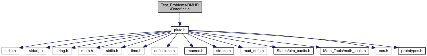
Go to the source code of this file.
Functions | |
| void | Init (double *v, double x1, double x2, double x3) |
| void | Analysis (const Data *d, Grid *grid) |
| void | UserDefBoundary (const Data *d, RBox *box, int side, Grid *grid) |
RMHD rotor test problem in 2 or 3 dimensions.
The 2D rotor problem [dZBL03][Mig12] consists of a rapidly spinning disk embedded in a uniform background medium treaded by a costant magnetic field. The initial conditin reads as
![\[ \left(\rho, p, v_x, v_y, B_x\right) = \left\{\begin{array}{ll} \left(10, 1,-\omega y,\,\omega x,\, 1\right) & \quad\mathrm{for}\quad r < 0.1 \\ \noalign{\medskip} \left(1,\, 1,\, 0,\, 0,\, 1\right) & \quad\mathrm{otherwise} \end{array}\right. \]](form_453.png)
where  is the angular frequency of rotation. The computational domain is the unit square and outflow boundary conditions are imposed everywhere.
As the disk rotates, strong torsional Alfven waves form and propagate outward carrying angular momentum from the disk to the ambient. The emerging flow structure is enclosed by a circular fast forward shock traveling into the surrounding medium. An inward fast shock bounds the innermost oval region where density has been depleted to lower values. The presence of the magnetic field slows down the rotor, and the maximum Lorentz factor decreases from the nominal value of 10 to 2.2 (approx).
A list of tested configurations is given in the following table:
| Conf. | GEOMETRY | DIM | T. STEPPING | RECONSTRUCTION | divB | AMR |
|---|---|---|---|---|---|---|
| #01 | CARTESIAN | 2 | RK3 | LINEAR | CT | NO |
| #02 | CARTESIAN | 2 | RK2 | LINEAR | CT | NO |
| #03 | CARTESIAN | 2 | HANCOCK | LINEAR | 8W | NO |
| #04 | CARTESIAN | 2 | HANCOCK | LINEAR | CT | NO |
| #05 | CARTESIAN | 3 | RK2 | LINEAR | GLM | NO |
| #06 | CARTESIAN | 3 | RK2 | LINEAR | GLM | NO |
| #07 | CARTESIAN | 3 | HANCOCK | LINEAR | CT | NO |
| #08 | CARTESIAN | 3 | RK3 | LimO3 | GLM | NO |
The final solutin at t = 0.4 on a grid of 400x400 grid points is shown below.

The three dimensional version extends the current configuration to a spinning sphere and it is described in [MUB09].
Reference:
Definition in file init.c.
| void Init | ( | double * | v, |
| double | x1, | ||
| double | x2, | ||
| double | x3 | ||
| ) |
The Init() function can be used to assign initial conditions as as a function of spatial position.
| [out] | v | a pointer to a vector of primitive variables |
| [in] | x1 | coordinate point in the 1st dimension |
| [in] | x2 | coordinate point in the 2nd dimension |
| [in] | x3 | coordinate point in the 3rdt dimension |
The meaning of x1, x2 and x3 depends on the geometry:
![\[ \begin{array}{cccl} x_1 & x_2 & x_3 & \mathrm{Geometry} \\ \noalign{\medskip} \hline x & y & z & \mathrm{Cartesian} \\ \noalign{\medskip} R & z & - & \mathrm{cylindrical} \\ \noalign{\medskip} R & \phi & z & \mathrm{polar} \\ \noalign{\medskip} r & \theta & \phi & \mathrm{spherical} \end{array} \]](form_173.png)
Variable names are accessed by means of an index v[nv], where nv = RHO is density, nv = PRS is pressure, nv = (VX1, VX2, VX3) are the three components of velocity, and so forth.
Definition at line 68 of file init.c.
Assign user-defined boundary conditions.
| [in,out] | d | pointer to the PLUTO data structure containing cell-centered primitive quantities (d->Vc) and staggered magnetic fields (d->Vs, when used) to be filled. |
| [in] | box | pointer to a RBox structure containing the lower and upper indices of the ghost zone-centers/nodes or edges at which data values should be assigned. |
| [in] | side | specifies the boundary side where ghost zones need to be filled. It can assume the following pre-definite values: X1_BEG, X1_END, X2_BEG, X2_END, X3_BEG, X3_END. The special value side == 0 is used to control a region inside the computational domain. |
| [in] | grid | pointer to an array of Grid structures. |
Assign user-defined boundary conditions in the lower boundary ghost zones. The profile is top-hat:
![\[ V_{ij} = \left\{\begin{array}{ll} V_{\rm jet} & \quad\mathrm{for}\quad r_i < 1 \\ \noalign{\medskip} \mathrm{Reflect}(V) & \quad\mathrm{otherwise} \end{array}\right. \]](form_235.png)
where  and
and M is the flow Mach number (the unit velocity is the jet sound speed, so  ).
).
Assign user-defined boundary conditions:
x < 1/6 and reflective boundary otherwise. we use fixed (post-shock) values. Unperturbed values otherwise.
Assign user-defined boundary conditions at inner and outer radial boundaries. Reflective conditions are applied except for the azimuthal velocity which is fixed.
Assign user-defined boundary conditions.
| [in/out] | d pointer to the PLUTO data structure containing cell-centered primitive quantities (d->Vc) and staggered magnetic fields (d->Vs, when used) to be filled. | |
| [in] | box | pointer to a RBox structure containing the lower and upper indices of the ghost zone-centers/nodes or edges at which data values should be assigned. |
| [in] | side | specifies on which side boundary conditions need to be assigned. side can assume the following pre-definite values: X1_BEG, X1_END, X2_BEG, X2_END, X3_BEG, X3_END. The special value side == 0 is used to control a region inside the computational domain. |
| [in] | grid | pointer to an array of Grid structures. |
Set the injection boundary condition at the lower z-boundary (X2-beg must be set to userdef in pluto.ini). For  we set constant input values (given by the GetJetValues() function while for $ R > 1 $ the solution has equatorial symmetry with respect to the
 z=0 plane. To avoid numerical problems with a "top-hat" discontinuous jump, we smoothly merge the inlet and reflected value using a profile function Profile().
Provide inner radial boundary condition in polar geometry. Zero gradient is prescribed on density, pressure and magnetic field. For the velocity, zero gradient is imposed on v/r (v = vr, vphi).
The user-defined boundary is used to impose stress-free boundary and purely vertical magnetic field at the top and bottom boundaries, as done in Bodo et al. (2012). In addition, constant temperature and hydrostatic balance are imposed. For instance, at the bottom boundary, one has:
![\[ \left\{\begin{array}{lcl} \DS \frac{dp}{dz} &=& \rho g_z \\ \noalign{\medskip} p &=& \rho c_s^2 \end{array}\right. \qquad\Longrightarrow\qquad \frac{p_{k+1}-p_k}{\Delta z} = \frac{p_{k} + p_{k+1}}{2c_s^2}g_z \]](form_395.png)
where  is the value of gravity at the lower boundary. Solving for
  at the bottom boundary where
  gives:
![\[ \left\{\begin{array}{lcl} p_k &=& \DS p_{k+1} \frac{1-a}{1+a} \\ \noalign{\medskip} \rho_k &=& \DS \frac{p_k}{c_s^2} \end{array}\right. \qquad\mathrm{where}\qquad a = \frac{\Delta z g_z}{2c_s^2} > 0 \]](form_399.png)
where, for simplicity, we keep constant temperature in the ghost zones rather than at the boundary interface (this seems to give a more stable behavior and avoids negative densities). A similar treatment holds at the top boundary.
Assign user-defined boundary conditions. At the inner boundary we use outflow conditions, except for velocity which we reset to zero when there's an inflow
Definition at line 135 of file init.c.
 1.8.10
