|
PLUTO
|
Relativistic magnetized jet in axisymmetric coordinates. More...
#include "pluto.h"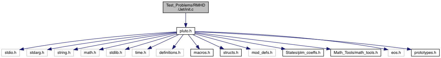
Go to the source code of this file.
Functions | |
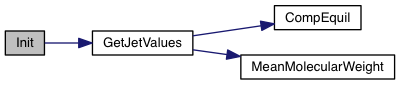
| static void | GetJetValues (double x1, double x2, double x3, double *vj) |
| void | Init (double *v, double x1, double x2, double x3) |
| void | Analysis (const Data *d, Grid *grid) |
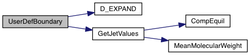
| void | UserDefBoundary (const Data *d, RBox *box, int side, Grid *grid) |
Variables | |
| static double | pj |
| static double | g_gamma |
Relativistic magnetized jet in axisymmetric coordinates.
The jet problem is set up in axisymmetric cylindrical coordinates  as described in section 4.2.3 of Mignone, Ugliano & Bodo (2009, [MUB09] hereafter). We label ambient and jet values with the suffix "a" and "j", respectively. The ambient medium is at rest and is characterized by uniform density and pressure,
  and
and  . The beam enters from the lower-z boundary from a circular nozzle of radius 1, carries a constant poloidal field
  and a (radially-varying) toroidal component
  . Flow variables are prescribed as
![\[ \left\{\begin{array}{lcl} \rho(R) &=& \rho_j \\ \noalign{\medskip} v_z(R) &=& v_j \\ \noalign{\medskip} B_\phi(R) &=& \DS \left\{\begin{array}{ll} -\gamma_j b_m R/a & \quad{\rm for}\quad r<a \\ \noalign{\medskip} -\gamma_j b_m a/R & \quad{\rm for}\quad r>a \end{array}\right. \\ \noalign{\medskip} B_z(R) &=& B_{z0}\quad\mathrm{(const)} \end{array}\right. \]](form_437.png)
Here a is the magnetization radius while  . The pressure distribution is found by solving the radial momentum balance between thermal, centrifugal and magnetic forces. Neglecting rotation and assuming
 Bz to be constant the solution is given by
![\[ p(R) = p_j + b_m^2\left[1-\min\left(\frac{r^2}{a^2},1\right)\right] \]](form_439.png)
Here  is the jet/ambient pressure at
 r=1 and its value depends on the Mach number, see [MUB09].
The parameters controlling the problem is
g_inputParam[MACH]: the jet Mach number  where
where  is the sound speed and
  . This is used to recover
  ;
;g_inputParam[LORENTZ]: the jet Lorentz factor;g_inpurParam[RHOJ]: the jet density;g_inpurParam[SIGMA_POL]: magnetization strength for poloidal magnetic field component (see [MUB09], Eq [65]);g_inpurParam[SIGMA_TOR]: magnetization strength for toroidal magnetic field component (see [MUB09], Eq [65]);The different configurations are:
The following image show the (log) density map at the end of simulation for setup #01.

References
Definition in file init.c.
|
static |
Definition at line 183 of file init.c.
| void Init | ( | double * | v, |
| double | x1, | ||
| double | x2, | ||
| double | x3 | ||
| ) |
The Init() function can be used to assign initial conditions as as a function of spatial position.
| [out] | v | a pointer to a vector of primitive variables |
| [in] | x1 | coordinate point in the 1st dimension |
| [in] | x2 | coordinate point in the 2nd dimension |
| [in] | x3 | coordinate point in the 3rdt dimension |
The meaning of x1, x2 and x3 depends on the geometry:
![\[ \begin{array}{cccl} x_1 & x_2 & x_3 & \mathrm{Geometry} \\ \noalign{\medskip} \hline x & y & z & \mathrm{Cartesian} \\ \noalign{\medskip} R & z & - & \mathrm{cylindrical} \\ \noalign{\medskip} R & \phi & z & \mathrm{polar} \\ \noalign{\medskip} r & \theta & \phi & \mathrm{spherical} \end{array} \]](form_173.png)
Variable names are accessed by means of an index v[nv], where nv = RHO is density, nv = PRS is pressure, nv = (VX1, VX2, VX3) are the three components of velocity, and so forth.
Definition at line 80 of file init.c.
Assign user-defined boundary conditions.
| [in,out] | d | pointer to the PLUTO data structure containing cell-centered primitive quantities (d->Vc) and staggered magnetic fields (d->Vs, when used) to be filled. |
| [in] | box | pointer to a RBox structure containing the lower and upper indices of the ghost zone-centers/nodes or edges at which data values should be assigned. |
| [in] | side | specifies the boundary side where ghost zones need to be filled. It can assume the following pre-definite values: X1_BEG, X1_END, X2_BEG, X2_END, X3_BEG, X3_END. The special value side == 0 is used to control a region inside the computational domain. |
| [in] | grid | pointer to an array of Grid structures. |
Assign user-defined boundary conditions in the lower boundary ghost zones. The profile is top-hat:
![\[ V_{ij} = \left\{\begin{array}{ll} V_{\rm jet} & \quad\mathrm{for}\quad r_i < 1 \\ \noalign{\medskip} \mathrm{Reflect}(V) & \quad\mathrm{otherwise} \end{array}\right. \]](form_235.png)
where  and
and M is the flow Mach number (the unit velocity is the jet sound speed, so  ).
).
Assign user-defined boundary conditions:
x < 1/6 and reflective boundary otherwise. we use fixed (post-shock) values. Unperturbed values otherwise.
Assign user-defined boundary conditions at inner and outer radial boundaries. Reflective conditions are applied except for the azimuthal velocity which is fixed.
Assign user-defined boundary conditions.
| [in/out] | d pointer to the PLUTO data structure containing cell-centered primitive quantities (d->Vc) and staggered magnetic fields (d->Vs, when used) to be filled. | |
| [in] | box | pointer to a RBox structure containing the lower and upper indices of the ghost zone-centers/nodes or edges at which data values should be assigned. |
| [in] | side | specifies on which side boundary conditions need to be assigned. side can assume the following pre-definite values: X1_BEG, X1_END, X2_BEG, X2_END, X3_BEG, X3_END. The special value side == 0 is used to control a region inside the computational domain. |
| [in] | grid | pointer to an array of Grid structures. |
Set the injection boundary condition at the lower z-boundary (X2-beg must be set to userdef in pluto.ini). For  we set constant input values (given by the GetJetValues() function while for $ R > 1 $ the solution has equatorial symmetry with respect to the
 z=0 plane. To avoid numerical problems with a "top-hat" discontinuous jump, we smoothly merge the inlet and reflected value using a profile function Profile().
Provide inner radial boundary condition in polar geometry. Zero gradient is prescribed on density, pressure and magnetic field. For the velocity, zero gradient is imposed on v/r (v = vr, vphi).
The user-defined boundary is used to impose stress-free boundary and purely vertical magnetic field at the top and bottom boundaries, as done in Bodo et al. (2012). In addition, constant temperature and hydrostatic balance are imposed. For instance, at the bottom boundary, one has:
![\[ \left\{\begin{array}{lcl} \DS \frac{dp}{dz} &=& \rho g_z \\ \noalign{\medskip} p &=& \rho c_s^2 \end{array}\right. \qquad\Longrightarrow\qquad \frac{p_{k+1}-p_k}{\Delta z} = \frac{p_{k} + p_{k+1}}{2c_s^2}g_z \]](form_395.png)
where  is the value of gravity at the lower boundary. Solving for
  at the bottom boundary where
  gives:
![\[ \left\{\begin{array}{lcl} p_k &=& \DS p_{k+1} \frac{1-a}{1+a} \\ \noalign{\medskip} \rho_k &=& \DS \frac{p_k}{c_s^2} \end{array}\right. \qquad\mathrm{where}\qquad a = \frac{\Delta z g_z}{2c_s^2} > 0 \]](form_399.png)
where, for simplicity, we keep constant temperature in the ghost zones rather than at the boundary interface (this seems to give a more stable behavior and avoids negative densities). A similar treatment holds at the top boundary.
Assign user-defined boundary conditions. At the inner boundary we use outflow conditions, except for velocity which we reset to zero when there's an inflow
Definition at line 128 of file init.c.
 1.8.10
