|
PLUTO
|
Magnetized accretion torus. More...
#include "pluto.h"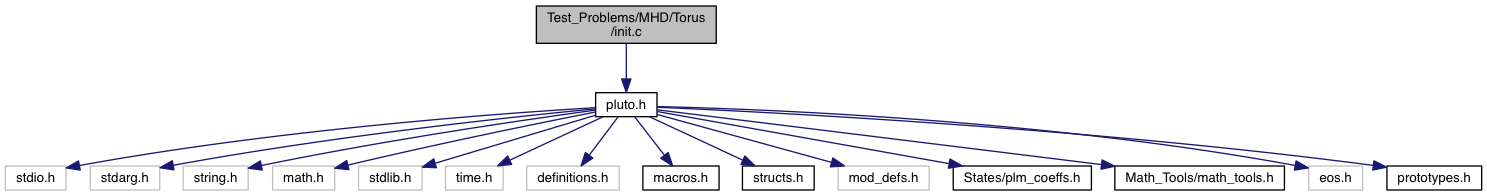
Go to the source code of this file.
Functions | |
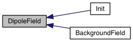
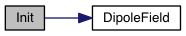
| static void | DipoleField (double x1, double x2, double x3, double *Bx1, double *Bx2, double *A) |
| void | Init (double *v, double x1, double x2, double x3) |
| void | Analysis (const Data *d, Grid *grid) |
| void | BackgroundField (double x1, double x2, double x3, double *B0) |
| void | UserDefBoundary (const Data *d, RBox *box, int side, Grid *grid) |
Variables | |
| static double | kappa |
Magnetized accretion torus.
Magnetized accretion torus in 2D spherical coordinates in a radially stratified atmosphere. The accretion torus is determined by the equilibrium condition
![\[ -\frac{1}{R} + \frac{1}{2(1-a)}\frac{L_k^2}{r^{2-2a}} +(n+1)\frac{p}{\rho} = const \]](form_411.png)
where  ,
, R is the spherical radius, r is the cylindrical radius. Since  then
then  we can also write using
  (constant angular momentum distribution, Kuwabara Eq [8]):
![\[ -\frac{1}{R} + \frac{1}{2}\frac{L_k^2}{r^2} + \frac{\gamma}{\gamma-1}K\rho^{\gamma-1} = c = -\frac{1}{r_{\min}} + \frac{1}{2}\frac{L_k^2}{r_{\min}^2} \]](form_416.png)
where the constant on the right hand side is determined at the zero pressure surface. The previous equation is used to compute K at the point where the density is maximum and then again to obtain the density distribution:
![\[ K = \frac{\gamma-1}{\gamma}\left[ c + \frac{1}{r_{\max}} - \frac{1}{2}\frac{L_k^2}{r_{\max}^2} \right]\frac{1}{\rho_{\max}^{\gamma-1}}\,;\qquad \rho = \left[\frac{\gamma-1}{K\gamma}\left(c + \frac{1}{R} - \frac{1}{2}\frac{L_k^2}{r^2}\right)\right]^{1/(\gamma-1)} \]](form_417.png)
Thus, specifying  ,
,  and
and  determine the torus structure completely. The torus azimuthal velocity is compute from
  .
.
The atmosphere is assumed to be isothermal and it is given by the condition of hydrostatic balance:
![\[ \rho_a(R) = \eta\rho_{\max} \exp\left[\left(\frac{1}{R}-\frac{1}{r_{\min}}\right) \frac{GM}{a^2}\right] \]](form_422.png)
where  is the density contrast between the (maximum) torus density and the atmosphere density at
  .
.
The torus surface is defined by the condition  .
.
The dimensionless form of the equation employs on the following units:
![$ [\rho] = \rho_{\max}$](form_425.png) : reference density;
: reference density;![$ [L] = R_{*} $](form_426.png) : star radius;
: star radius;![$ [v^2] = GM/L $](form_427.png) : reference (squared) velocity.
: reference (squared) velocity.The user defined parameters of this problem, as they appear in pluto.ini, allows for control in the Torus shape and the contrast of physical values:
g_inputParam[RMIN]: minimum cylindrical radius for the torus (inner rim)g_inputParam[RMAX]: radius of the Torus where pressure is maximumg_inputParam[RHO_CUT]: minimum density to define the last contour of the magnetic vec. pot.g_inputParam[BETA]: plasma betag_inputParam[ETA] density contrast between atmosphere and Torusg_inputParam[SCALE_HEIGHT]: atmosphere scale height 
The magnetic field can be specified to be inside the torus or as a large-scale dipole field. In the first case, we give the vector potential:
![\[ A_\phi = B_0(\rho_t - \rho_{\rm cut}) \]](form_429.png)
In the second case, a dipole field is specified in the function DipoleField(). The user-defined constant USE_DIPOLE can be used to select between the two configurations.
References
Definition in file init.c.
| void BackgroundField | ( | double | x1, |
| double | x2, | ||
| double | x3, | ||
| double * | B0 | ||
| ) |
Define the component of a static, curl-free background magnetic field.
Definition at line 212 of file init.c.

|
static |
Assign the polodial component of magnetic fields and vector potential for a dipole.
Definition at line 300 of file init.c.
| void Init | ( | double * | v, |
| double | x1, | ||
| double | x2, | ||
| double | x3 | ||
| ) |
The Init() function can be used to assign initial conditions as as a function of spatial position.
| [out] | v | a pointer to a vector of primitive variables |
| [in] | x1 | coordinate point in the 1st dimension |
| [in] | x2 | coordinate point in the 2nd dimension |
| [in] | x3 | coordinate point in the 3rdt dimension |
The meaning of x1, x2 and x3 depends on the geometry:
![\[ \begin{array}{cccl} x_1 & x_2 & x_3 & \mathrm{Geometry} \\ \noalign{\medskip} \hline x & y & z & \mathrm{Cartesian} \\ \noalign{\medskip} R & z & - & \mathrm{cylindrical} \\ \noalign{\medskip} R & \phi & z & \mathrm{polar} \\ \noalign{\medskip} r & \theta & \phi & \mathrm{spherical} \end{array} \]](form_173.png)
Variable names are accessed by means of an index v[nv], where nv = RHO is density, nv = PRS is pressure, nv = (VX1, VX2, VX3) are the three components of velocity, and so forth.
Definition at line 104 of file init.c.
Assign user-defined boundary conditions. At the inner boundary we use outflow conditions, except for velocity which we reset to zero when there's an inflow
Definition at line 230 of file init.c.
 1.8.10
