|
PLUTO
|
Magnetic field diffusion in 2D and 3D. More...
#include "pluto.h"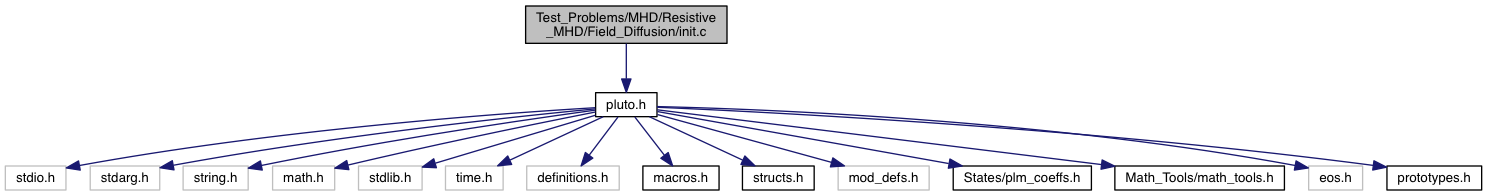
Go to the source code of this file.
Functions | |
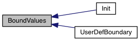
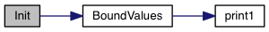
| void | BoundValues (double *v, double x1, double x2, double x3, double t) |
| void | Init (double *us, double x1, double x2, double x3) |
| void | Analysis (const Data *d, Grid *grid) |
| void | UserDefBoundary (const Data *d, RBox *box, int side, Grid *grid) |
Magnetic field diffusion in 2D and 3D.
Sets the initial conditions for a magnetic field diffusion problem in 2 or 3 dimensions. This is a useful test to check the ability of the code to solve standard diffusion problems. The magnetic field has initially a Gaussian profile, and an anisotropic resistivity is possible. This problem has an analytical solution given, in 2D, by
![\[ B_x(y,t) = \exp(-y^2/4\eta_zt)/\sqrt{t} \quad\quad\quad B_y(x,t) = \exp(-x^2/4\eta_zt)/\sqrt{t} \quad\quad\quad B_z(x,y,t) = \exp(-x^2/4\eta_yt)\exp(-y^2/4\eta_xt)/t \]](form_374.png)
and in 3D by
![\[ \begin{array}{lcl} B_x(y,z,t) &=& \exp(-y^2/4\eta_zt)\exp(-z^2/4\eta_yt)/t \\ \noalign{\medskip} B_y(x,z,t) &=& \exp(-x^2/4\eta_zt)\exp(-z^2/4\eta_xt)/t \\ \noalign{\medskip} B_z(x,y,t) &=& \exp(-x^2/4\eta_yt)\exp(-y^2/4\eta_xt)/t \end{array} \]](form_375.png)
The initial condition is simply set using the previous profiles with t=1. In order to solve only the parabolic term in the induction equation (  ) we give to the fluid a very large intertia using a high density value. Moreover, to avoid any fluid motion, the velocity is reset to zero at each time step by using the
 INTERNAL_BOUNDARY.
The runtime parameters that are read from pluto.ini are
g_inputParam[ETAX]: sets the resistivity along the  direction;
g_inputParam[ETAY]: sets the resistivity along the  direction;
g_inputParam[ETAZ]: sets the resistivity along the  direction;
The configurations use both EXPLICIT and STS time integrators and different geometries are explored:
| Conf. | GEOMETRY | DIM | T.STEPPING | divB | RESISTIVITY |
|---|---|---|---|---|---|
| #01 | CARTESIAN | 3 | RK2 | 8W | EXPLICIT |
| #02 | CARTESIAN | 3 | HANCOCK | GLM | STS |
| #03 | CARTESIAN | 3 | RK3 | CT | EXPLICIT |
| #04 | CARTESIAN | 3 | HANCOCK | GLM | EXPLICIT |
| #05 | POLAR | 3 | RK2 | 8W | EXPLICIT |
| #06 | POLAR | 3 | RK2 | 8W | STS |
| #07 | SPHERICAL | 3 | RK2 | 8W | EXPLICIT |
| #08 | SPHERICAL | 3 | RK2 | 8W | STS |
| #09 | SPHERICAL | 3 | RK3 | CT | EXPLICIT |
| #10 | CARTESIAN | 2 | HANCOCK | CT | EXPLICIT |
| #11 | CARTESIAN | 3 | HANCOCK | CT | EXPLICIT |
| #12 | CARTESIAN | 2 | HANCOCK | CT | STS |
| #13 | SPHERICAL | 3 | RK2 | CT | STS |
Definition in file init.c.
| void BoundValues | ( | double * | v, |
| double | x1, | ||
| double | x2, | ||
| double | x3, | ||
| double | t | ||
| ) |
Definition at line 158 of file init.c.

| void Init | ( | double * | us, |
| double | x1, | ||
| double | x2, | ||
| double | x3 | ||
| ) |
The Init() function can be used to assign initial conditions as as a function of spatial position.
| [out] | v | a pointer to a vector of primitive variables |
| [in] | x1 | coordinate point in the 1st dimension |
| [in] | x2 | coordinate point in the 2nd dimension |
| [in] | x3 | coordinate point in the 3rdt dimension |
The meaning of x1, x2 and x3 depends on the geometry:
![\[ \begin{array}{cccl} x_1 & x_2 & x_3 & \mathrm{Geometry} \\ \noalign{\medskip} \hline x & y & z & \mathrm{Cartesian} \\ \noalign{\medskip} R & z & - & \mathrm{cylindrical} \\ \noalign{\medskip} R & \phi & z & \mathrm{polar} \\ \noalign{\medskip} r & \theta & \phi & \mathrm{spherical} \end{array} \]](form_173.png)
Variable names are accessed by means of an index v[nv], where nv = RHO is density, nv = PRS is pressure, nv = (VX1, VX2, VX3) are the three components of velocity, and so forth.
Definition at line 75 of file init.c.
Assign user-defined boundary conditions.
| [in,out] | d | pointer to the PLUTO data structure containing cell-centered primitive quantities (d->Vc) and staggered magnetic fields (d->Vs, when used) to be filled. |
| [in] | box | pointer to a RBox structure containing the lower and upper indices of the ghost zone-centers/nodes or edges at which data values should be assigned. |
| [in] | side | specifies the boundary side where ghost zones need to be filled. It can assume the following pre-definite values: X1_BEG, X1_END, X2_BEG, X2_END, X3_BEG, X3_END. The special value side == 0 is used to control a region inside the computational domain. |
| [in] | grid | pointer to an array of Grid structures. |
Assign user-defined boundary conditions in the lower boundary ghost zones. The profile is top-hat:
![\[ V_{ij} = \left\{\begin{array}{ll} V_{\rm jet} & \quad\mathrm{for}\quad r_i < 1 \\ \noalign{\medskip} \mathrm{Reflect}(V) & \quad\mathrm{otherwise} \end{array}\right. \]](form_235.png)
where  and
and M is the flow Mach number (the unit velocity is the jet sound speed, so  ).
).
Assign user-defined boundary conditions:
x < 1/6 and reflective boundary otherwise. we use fixed (post-shock) values. Unperturbed values otherwise.
Assign user-defined boundary conditions at inner and outer radial boundaries. Reflective conditions are applied except for the azimuthal velocity which is fixed.
Assign user-defined boundary conditions.
| [in/out] | d pointer to the PLUTO data structure containing cell-centered primitive quantities (d->Vc) and staggered magnetic fields (d->Vs, when used) to be filled. | |
| [in] | box | pointer to a RBox structure containing the lower and upper indices of the ghost zone-centers/nodes or edges at which data values should be assigned. |
| [in] | side | specifies on which side boundary conditions need to be assigned. side can assume the following pre-definite values: X1_BEG, X1_END, X2_BEG, X2_END, X3_BEG, X3_END. The special value side == 0 is used to control a region inside the computational domain. |
| [in] | grid | pointer to an array of Grid structures. |
Set the injection boundary condition at the lower z-boundary (X2-beg must be set to userdef in pluto.ini). For  we set constant input values (given by the GetJetValues() function while for $ R > 1 $ the solution has equatorial symmetry with respect to the
 z=0 plane. To avoid numerical problems with a "top-hat" discontinuous jump, we smoothly merge the inlet and reflected value using a profile function Profile().
Definition at line 91 of file init.c.

 1.8.10
