PLUTO
init.c File Reference

Accretion disk in 3D spherical coordinates. More...

#include "pluto.h"
Include dependency graph for init.c:

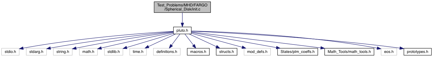
Go to the source code of this file.

Functions

void Init (double *us, double x1, double x2, double x3)
 
void Analysis (const Data *d, Grid *grid)
 
void UserDefBoundary (const Data *d, RBox *box, int side, Grid *grid)
 

Detailed Description

Accretion disk in 3D spherical coordinates.

Setup a magnetized disk in 3D spherical coordinates $(r,\theta,\phi$). The disk model is taken form [Flo11],[Mig12] and it consists of an initial equilibrium in a point mass gravity $ 1/r^2$ with equilibrium profiles given by

\[ \rho = \frac{1}{R^{3/2}}\exp\left[\frac{\sin(\theta) - 1}{c_0^2}\right] \,,\qquad p = c_s^2\rho\ ,,\qquad v_\phi = \frac{1}{\sqrt{r}}\left(1 - \frac{5}{2\sin\theta}c_0^2\right) \]

where $R = r\sin\theta$ is the cylindrical radius while $c_0 = H/R$ and $c_s = H/R^{3/2}$ is the sound speed. Here H is the scale height and it is proportional to the cylindrical radius. The constant of proportionality is the ratio $ H/R $ defined by the input parameter g_inputParam[H_R]. With the current setting, one rotation period of the inner orbit (r=1) is $\Delta T = 2\pi$.

Differently from [Flo11], a polodial magnetic field is used here, with vector potential prescribed as follows:

\[ A_\phi = A_0\frac{\sin(2\pi R) - R\cos(2\pi R)}{R} \exp\left[-\left(\frac{z}{H}\right)^4\right] \exp\left[-\left(\frac{R-6}{2}\right)^4\right] \]

where A0 is a constant chosen to prescribe a given plasma beta. The exponential terms on the right hand side confine the magnetic field in the midplane around R=6. We also make the vector potential vanish identically for $ z/H > 2.5$ or $ R < 2.5$.

The boundary conditions are all set to userdef:

  • at the inner radial boundary, zero-gradient is imposed except for the azimuthal velocity (which is fixed the equilibrium value) and the radial velocity which is zero if velocity is directed inside the domain or copied otherwise (this is referred to as the "diode" b.c.)
  • at the outer radial boundary we impose zero-gradient except for the azimuthal velocity (fixed to equil. value) and radial velocity which is reflected.
  • at the vertical (theta) boundaries, ghost zones are filled with the initial equilibrium solution.

For the sake of simplicity only a quarter of a disk is considered. This test problems can be run normally or using the FARGO module, giving a saving factor of (roughly) 5. The figure below was produced by running the current setup at twice the resolution and for 90 orbits using FARGO.

mhd_spherical_disk.02.png
Density map of the disk after 90 innter orbits at twice the resolution.
Authors
A. Mignone (migno.nosp@m.ne@p.nosp@m.h.uni.nosp@m.to.i.nosp@m.t)
Date
Aug 16, 2012

References

  • [Flo11]: "Turbulence and Steady Flows in 3D Global Stratified MHD Simulations of Accretion Disks", Flock et al., ApJ (2011), 735:122
  • [Mig12]: "A Conservative orbital advection scheme for simulations of magnetized shear flows with the PLUTO code", Mignone et al, A&A (2012) 545, A152

Definition in file init.c.

Function Documentation

void Analysis ( const Data d,
Grid grid 
)

Perform runtime data analysis.

Parameters
[in]dthe PLUTO Data structure
[in]gridpointer to array of Grid structures

Definition at line 109 of file init.c.

114 {
115  int i,j,k,nv;
116  static int first_call = 1;
117  double v[NVAR];
118  double *r, *th, *dVr, *dVth, *dVphi, vol;
119  double pm, kin;
120  double pmtot, Tmtot;
121  static double voltot;
122  FILE *fp;
123 
124  r = grid[IDIR].x;
125  th = grid[JDIR].x;
126  dVr = grid[IDIR].dV; dVth = grid[JDIR].dV; dVphi = grid[KDIR].dV;
127 
128 /* ---------------------------------------------------------
129  compute total volume once at the beginning
130  --------------------------------------------------------- */
131 
132  if (first_call){
133  voltot = 0.0;
134  DOM_LOOP(k,j,i) voltot += dVr[i]*dVth[j]*dVphi[k];
135  #ifdef PARALLEL
136  MPI_Allreduce (&voltot, &kin, 1, MPI_DOUBLE, MPI_SUM, MPI_COMM_WORLD);
137  MPI_Barrier (MPI_COMM_WORLD);
138  voltot = kin;
139  #endif
140  }
141 
142 /* --------------------------------------------------------
143  compute volume averages
144  -------------------------------------------------------- */
145 
146  pmtot = Tmtot = 0.0;
147  DOM_LOOP(k,j,i){
148  vol = dVr[i]*dVth[j]*dVphi[k]/voltot;
149 
150  for (nv = NVAR; nv--; ) v[nv] = d->Vc[nv][k][j][i];
151 
152  #if PHYSICS == MHD
153  pm = 0.5*(v[BX1]*v[BX1] + v[BX2]*v[BX2] + v[BX3]*v[BX3]);
154  pmtot += pm*vol;
155  Tmtot += v[BX1]*v[BX3]*vol;
156  #endif
157  }
158 
159  #ifdef PARALLEL
160  MPI_Allreduce (&pmtot, &vol, 1, MPI_DOUBLE, MPI_SUM, MPI_COMM_WORLD);
161  pmtot = vol;
162 
163  MPI_Allreduce (&Tmtot, &vol, 1, MPI_DOUBLE, MPI_SUM, MPI_COMM_WORLD);
164  Tmtot = vol;
165 
166  MPI_Barrier (MPI_COMM_WORLD);
167  #endif
168 
169 /* -----------------------------------------------------
170  Write "averages.dat" to disk.
171  The file is created as new if this is the very
172  initial time step. Data is appended otherwise.
173  Processor #0 does the actual writing.
174  ----------------------------------------------------- */
175 
176  if (prank == 0){
177  static double tpos = -1.0;
178  if (g_stepNumber == 0){
179  fp = fopen("averages.dat","w");
180  fprintf (fp,"#%s %12s %12s %12s\n",
181  " t","dt","<B^2>/2","<Tm>");
182  }else{
183  if (tpos < 0.0){ /* obtain time coordinate of to last entry */
184  char sline[512];
185  fp = fopen("averages.dat","r");
186  while (fgets(sline, 512, fp)) {}
187  sscanf(sline, "%lf\n",&tpos);
188  fclose(fp);
189  }
190  fp = fopen("averages.dat","a");
191  }
192  if (g_time > tpos){
193  fprintf (fp, "%12.6e %12.6e %12.6e %12.6e\n",
194  g_time, g_dt, pmtot, Tmtot);
195  }
196  fclose(fp);
197  }
198  first_call = 0;
199 }
DOM_LOOP(k, j, i)
Definition: analysis.c:22
double **** Vc
The main four-index data array used for cell-centered primitive variables.
Definition: structs.h:31
double g_dt
The current integration time step.
Definition: globals.h:118
double * dV
Cell volume.
Definition: structs.h:86
int prank
Processor rank.
Definition: globals.h:33
#define KDIR
Definition: pluto.h:195
long int g_stepNumber
Gives the current integration step number.
Definition: globals.h:97
#define IDIR
Definition: pluto.h:193
#define PHYSICS
Definition: definitions_01.h:1
int j
Definition: analysis.c:2
int k
Definition: analysis.c:2
double * x
Definition: structs.h:80
#define MHD
Definition: pluto.h:111
#define BX3
Definition: mod_defs.h:27
int i
Definition: analysis.c:2
double g_time
The current integration time.
Definition: globals.h:117
FILE * fp
Definition: analysis.c:7
#define BX1
Definition: mod_defs.h:25
#define BX2
Definition: mod_defs.h:26
#define JDIR
Definition: pluto.h:194
#define NVAR
Definition: pluto.h:609

Here is the call graph for this function:

void Init ( double *  us,
double  x1,
double  x2,
double  x3 
)

The Init() function can be used to assign initial conditions as as a function of spatial position.

Parameters
[out]va pointer to a vector of primitive variables
[in]x1coordinate point in the 1st dimension
[in]x2coordinate point in the 2nd dimension
[in]x3coordinate point in the 3rdt dimension

The meaning of x1, x2 and x3 depends on the geometry:

\[ \begin{array}{cccl} x_1 & x_2 & x_3 & \mathrm{Geometry} \\ \noalign{\medskip} \hline x & y & z & \mathrm{Cartesian} \\ \noalign{\medskip} R & z & - & \mathrm{cylindrical} \\ \noalign{\medskip} R & \phi & z & \mathrm{polar} \\ \noalign{\medskip} r & \theta & \phi & \mathrm{spherical} \end{array} \]

Variable names are accessed by means of an index v[nv], where nv = RHO is density, nv = PRS is pressure, nv = (VX1, VX2, VX3) are the three components of velocity, and so forth.

Definition at line 72 of file init.c.

76 {
77  static int first_call = 1;
78  double rnd, s, c, R, r, z;
79  double H, c0, cs, Bphi;
80 
81  g_gamma = 1.0001;
82  r = x1;
83  s = sin(x2);
84  c = cos(x2);
85 
86  R = r*s; /* Cylindrical radius */
87  z = r*c;
88  c0 = g_inputParam[H_R];
89  cs = c0/sqrt(R);
90  H = g_inputParam[H_R]*R;
91 
92  us[RHO] = exp((s-1.0)/(c0*c0))/(R*sqrt(R));
93  us[iVR] = 0.0;
94  us[iVTH] = 1.e-4*cs*cos(8.0*x3)*exp(-2.0*z*z/(H*H)); /* Perturbation */
95  us[iVPHI] = 1.0/sqrt(r)*(1.0 - 2.5*c0*c0/s);
96  us[PRS] = cs*cs*us[RHO];
97 
98  #if PHYSICS == MHD
99  us[BX1] = us[BX2] = us[BX3] = 0.0;
100  us[AX1] = us[AX2] = us[AX3] = 0.0;
101 
102  us[AX3] = (sin(2.0*CONST_PI*R) - R*cos(2.0*CONST_PI*R))/R;
103  us[AX3] *= 3.5e-4*exp(-pow(z/H,4.0))*exp(-pow((R-6.0)/2.0,4.0));
104  if (fabs(z/H) > 2.5 || R < 2.5) us[AX3] = 0.0;
105  #endif
106  g_smallPressure = 1.e-9;
107 }
double g_gamma
Definition: globals.h:112
#define RHO
Definition: mod_defs.h:19
#define iVPHI
Definition: mod_defs.h:67
#define AX2
Definition: mod_defs.h:86
double g_smallPressure
Small value for pressure fix.
Definition: globals.h:110
#define iVR
Definition: mod_defs.h:65
#define AX3
Definition: mod_defs.h:87
double g_inputParam[32]
Array containing the user-defined parameters.
Definition: globals.h:131
#define iVTH
Definition: mod_defs.h:66
tuple c
Definition: menu.py:375
#define H_R
#define s
#define BX3
Definition: mod_defs.h:27
#define AX1
Definition: mod_defs.h:85
#define BX1
Definition: mod_defs.h:25
#define CONST_PI
.
Definition: pluto.h:269
#define BX2
Definition: mod_defs.h:26
void UserDefBoundary ( const Data d,
RBox box,
int  side,
Grid grid 
)

Assign user-defined boundary conditions.

Parameters
[in,out]dpointer to the PLUTO data structure containing cell-centered primitive quantities (d->Vc) and staggered magnetic fields (d->Vs, when used) to be filled.
[in]boxpointer to a RBox structure containing the lower and upper indices of the ghost zone-centers/nodes or edges at which data values should be assigned.
[in]sidespecifies the boundary side where ghost zones need to be filled. It can assume the following pre-definite values: X1_BEG, X1_END, X2_BEG, X2_END, X3_BEG, X3_END. The special value side == 0 is used to control a region inside the computational domain.
[in]gridpointer to an array of Grid structures.

Assign user-defined boundary conditions in the lower boundary ghost zones. The profile is top-hat:

\[ V_{ij} = \left\{\begin{array}{ll} V_{\rm jet} & \quad\mathrm{for}\quad r_i < 1 \\ \noalign{\medskip} \mathrm{Reflect}(V) & \quad\mathrm{otherwise} \end{array}\right. \]

where $ V_{\rm jet} = (\rho,v,p)_{\rm jet} = (1,M,1/\Gamma)$ and M is the flow Mach number (the unit velocity is the jet sound speed, so $ v = M$).

Assign user-defined boundary conditions:

  • left side (x beg): constant shocked values
  • bottom side (y beg): constant shocked values for x < 1/6 and reflective boundary otherwise.
  • top side (y end): time-dependent boundary: for $ x < x_s(t) = 10 t/\sin\alpha + 1/6 + 1.0/\tan\alpha $ we use fixed (post-shock) values. Unperturbed values otherwise.

Assign user-defined boundary conditions at inner and outer radial boundaries. Reflective conditions are applied except for the azimuthal velocity which is fixed.

Assign user-defined boundary conditions.

Parameters
[in/out]d pointer to the PLUTO data structure containing cell-centered primitive quantities (d->Vc) and staggered magnetic fields (d->Vs, when used) to be filled.
[in]boxpointer to a RBox structure containing the lower and upper indices of the ghost zone-centers/nodes or edges at which data values should be assigned.
[in]sidespecifies on which side boundary conditions need to be assigned. side can assume the following pre-definite values: X1_BEG, X1_END, X2_BEG, X2_END, X3_BEG, X3_END. The special value side == 0 is used to control a region inside the computational domain.
[in]gridpointer to an array of Grid structures.

Definition at line 201 of file init.c.

207 {
208  int i, j, k, nv;
209  double c0, cs, qx, qy, qz, s, v[256];
210  double *r, *th, *phi;
211 
212  r = grid[IDIR].xgc;
213  th = grid[JDIR].xgc;
214  phi = grid[KDIR].xgc;
215  c0 = g_inputParam[H_R];
216 
217  if (side == 0) { /* -- check solution inside domain -- */
218  }
219 
220  if (side == X1_BEG){ /* -- X1_BEG boundary -- */
221  if (box->vpos == CENTER){
222  BOX_LOOP(box,k,j,i){
223  for (nv = 0; nv < NVAR; nv++) d->Vc[nv][k][j][i]= d->Vc[nv][k][j][IBEG];
224  s = sin(th[j]);
225  d->Vc[iVPHI][k][j][i] = 1.0/sqrt(r[i])*(1.0 - 2.5*c0*c0/s);
226  if (d->Vc[iVR][k][j][i] > 0.0) d->Vc[iVR][k][j][i] = 0.0;
227  }
228  }else if (box->vpos == X2FACE){
229  #ifdef STAGGERED_MHD
230  BOX_LOOP(box,k,j,i) d->Vs[BX2s][k][j][i] = d->Vs[BX2s][k][j][IBEG];
231  #endif
232  }else if (box->vpos == X3FACE){
233  #ifdef STAGGERED_MHD
234  BOX_LOOP(box,k,j,i) d->Vs[BX3s][k][j][i] = d->Vs[BX3s][k][j][IBEG];
235  #endif
236  }
237  }
238 
239  if (side == X1_END){ /* -- X1_END boundary -- */
240  if (box->vpos == CENTER){
241  BOX_LOOP(box, k, j, i){
242  for (nv = 0; nv < NVAR; nv++) d->Vc[nv][k][j][i]= d->Vc[nv][k][j][IEND];
243  s = sin(th[j]);
244  d->Vc[iVPHI][k][j][i] = 1.0/sqrt(r[i])*(1.0 - 2.5*c0*c0/s);
245  d->Vc[iVR][k][j][i] = -d->Vc[iVR][k][j][2*IEND - i + 1];
246  }
247  }else if (box->vpos == X2FACE){
248  #ifdef STAGGERED_MHD
249  BOX_LOOP(box,k,j,i) d->Vs[BX2s][k][j][i] = d->Vs[BX2s][k][j][IEND];
250  #endif
251  }else if (box->vpos == X3FACE){
252  #ifdef STAGGERED_MHD
253  BOX_LOOP(box,k,j,i) d->Vs[BX3s][k][j][i] = d->Vs[BX3s][k][j][IEND];
254  #endif
255  }
256  }
257 
258  if (side == X2_BEG){ /* -- X2_BEG boundary -- */
259  if (box->vpos == CENTER){
260  BOX_LOOP(box, k, j, i){
261  Init (v, r[i], th[j], phi[k]);
262  cs = c0/sqrt(r[i]*sin(th[j]));
263  v[iVTH] = 0.0;
264  v[PRS] = v[RHO]*cs*cs;
265  for (nv = 0; nv < NVAR; nv++) d->Vc[nv][k][j][i]= v[nv];
266  }
267  }else if (box->vpos == X1FACE){
268  #ifdef STAGGERED_MHD
269  BOX_LOOP(box, k, j, i) d->Vs[BX1s][k][j][i] = 0.0;
270  #endif
271  }else if (box->vpos == X3FACE){
272  #ifdef STAGGERED_MHD
273  BOX_LOOP(box, k, j, i) d->Vs[BX3s][k][j][i] = 0.0;
274  #endif
275  }
276 
277  }
278 
279  if (side == X2_END){ /* -- X2_END boundary -- */
280  if (box->vpos == CENTER){
281  BOX_LOOP(box, k, j, i){
282  Init (v, r[i], th[j], phi[k]);
283  cs = c0/sqrt(r[i]*sin(th[j]));
284  v[iVTH] = 0.0;
285  v[PRS] = v[RHO]*cs*cs;
286  for (nv = 0; nv < NVAR; nv++) d->Vc[nv][k][j][i]= v[nv];
287  }
288  }else if (box->vpos == X1FACE){
289  #ifdef STAGGERED_MHD
290  BOX_LOOP(box, k, j, i) d->Vs[BX1s][k][j][i] = 0.0;
291  #endif
292  }else if (box->vpos == X3FACE){
293  #ifdef STAGGERED_MHD
294  BOX_LOOP(box, k, j, i) d->Vs[BX3s][k][j][i] = 0.0;
295  #endif
296  }
297  }
298 }
#define X1_BEG
Boundary region at X1 beg.
Definition: pluto.h:146
#define CENTER
Definition: pluto.h:200
int vpos
Location of the variable inside the cell.
Definition: structs.h:359
#define RHO
Definition: mod_defs.h:19
#define X3FACE
Definition: pluto.h:203
#define BOX_LOOP(B, k, j, i)
Definition: macros.h:70
double **** Vc
The main four-index data array used for cell-centered primitive variables.
Definition: structs.h:31
#define iVPHI
Definition: mod_defs.h:67
#define BX3s
Definition: ct.h:29
#define X1_END
Boundary region at X1 end.
Definition: pluto.h:147
#define KDIR
Definition: pluto.h:195
#define X1FACE
Definition: pluto.h:201
#define iVR
Definition: mod_defs.h:65
#define IDIR
Definition: pluto.h:193
#define X2_END
Boundary region at X2 end.
Definition: pluto.h:149
double g_inputParam[32]
Array containing the user-defined parameters.
Definition: globals.h:131
int j
Definition: analysis.c:2
#define iVTH
Definition: mod_defs.h:66
long int IEND
Upper grid index of the computational domain in the the X1 direction for the local processor...
Definition: globals.h:37
int k
Definition: analysis.c:2
#define BX1s
Definition: ct.h:27
double * xgc
Cell volumetric centroid (!= x when geometry != CARTESIAN).
Definition: structs.h:84
#define H_R
#define s
int i
Definition: analysis.c:2
#define BX2s
Definition: ct.h:28
#define X2_BEG
Boundary region at X2 beg.
Definition: pluto.h:148
#define JDIR
Definition: pluto.h:194
#define NVAR
Definition: pluto.h:609
#define X2FACE
Definition: pluto.h:202
long int IBEG
Lower grid index of the computational domain in the the X1 direction for the local processor...
Definition: globals.h:35
void Init(double *v, double x1, double x2, double x3)
Definition: init.c:17

Here is the call graph for this function: