|
PLUTO
|
MHD blast wave. More...
#include "pluto.h"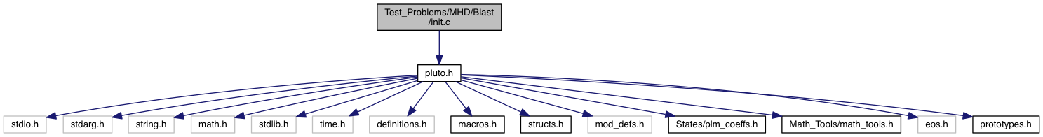
Go to the source code of this file.
Functions | |
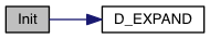
| void | Init (double *us, double x1, double x2, double x3) |
| void | Analysis (const Data *d, Grid *grid) |
| void | UserDefBoundary (const Data *d, RBox *box, int side, Grid *grid) |
| void | BackgroundField (double x1, double x2, double x3, double *B0) |
MHD blast wave.
The MHD blast wave problem has been specifically designed to show the scheme ability to handle strong shock waves propagating in highly magnetized environments. Depending on the strength of the magnetic field, it can become a rather arduous test leading to unphysical densities or pressures if the divergence-free condition is not adequately controlled and the numerical scheme does not introduce proper dissipation across curved shock fronts.
In this example the initial conditions consists of a static medium with uniform density  while pressure and magnetic field are given by
![\[ p = \left\{\begin{array}{ll} p_{\rm in} & \qquad\mathrm{for}\quad r < r_0 \\ \noalign{\medskip} p_{\rm out} & \qquad\mathrm{otherwise} \\ \end{array}\right.\,;\qquad \vec{B} = B_0\left( \sin\theta\cos\phi\hvec{x} + \sin\theta\sin\phi\hvec{y} + \cos\theta\hvec{z}\right) \]](form_275.png)
The values  are control parameters that can be changed from
 pluto.ini using, respectively,
g_inputParam[P_IN]g_inputParam[P_OUT]g_inputParam[BMAG]g_inputParam[THETA]g_inputParam[PHI]g_inputParam[RADIUS]The over-pressurized region drives a blast wave delimited by an outer fast forward shock propagating (nearly) radially while magnetic field lines pile up behind the shock thus building a region of higher magnetic pressure. In these regions the shock becomes magnetically dominated and only weakly compressive (  in both cases). The inner structure is delimited by an oval-shaped slow shock adjacent to a contact discontinuity and the two fronts tend to blend together as the propagation becomes perpendicular to the field lines. The magnetic energy increases behind the fast shock and decreases downstream of the slow shock. The resulting explosion becomes highly anisotropic and magnetically confined.
The available configurations are taken by collecting different setups available in literature:
| Conf. | GEOMETRY | DIM | T. STEP. | INTERP. | divB | BCK_FIELD | Ref |
|---|---|---|---|---|---|---|---|
| #01 | CARTESIAN | 2 | RK2 | LINEAR | CT | NO | [BS99] |
| #02 | CARTESIAN | 3 | RK2 | LINEAR | CT | NO | [Z04] |
| #03 | CYLINDRICAL | 2 | RK2 | LINEAR | CT | NO | [Z04] (*) |
| #04 | CYLINDRICAL | 2 | RK2 | LINEAR | CT | YES | [Z04] (*) |
| #05 | CARTESIAN | 3 | RK2 | LINEAR | CT | YES | [Z04] |
| #06 | CARTESIAN | 3 | ChTr | PARABOLIC | CT | NO | [GS08],[MT10] |
| #07 | CARTESIAN | 3 | ChTr | LINEAR | CT | NO | [GS08],[MT10] |
| #08 | CARTESIAN | 2 | ChTr | LINEAR | GLM | NO | [MT10] (2D version) |
| #09 | CARTESIAN | 3 | ChTr | LINEAR | GLM | NO | [GS08],[MT10] |
| #10 | CARTESIAN | 3 | RK2 | LINEAR | CT | YES | [Z04] |
| #11 | CARTESIAN | 3 | ChTr | LINEAR | EGLM | NO | [MT10] (**) |
(*) Setups are in different coordinates and with different orientation of magnetic field using constrained-transport MHD. (**) second version in sec. 4.7
The snapshot below show the solution for configuration #11.
This setup also works with the BACKGROUND_FIELD spliting. In this case the initial magnetic field is assigned in the BackgroundField() function while the Init() function is used to initialize the deviation to 0.


References:
Definition in file init.c.
| void BackgroundField | ( | double | x1, |
| double | x2, | ||
| double | x3, | ||
| double * | B0 | ||
| ) |
Define the component of a static, curl-free background magnetic field.
Definition at line 164 of file init.c.
| void Init | ( | double * | us, |
| double | x1, | ||
| double | x2, | ||
| double | x3 | ||
| ) |
The Init() function can be used to assign initial conditions as as a function of spatial position.
| [out] | v | a pointer to a vector of primitive variables |
| [in] | x1 | coordinate point in the 1st dimension |
| [in] | x2 | coordinate point in the 2nd dimension |
| [in] | x3 | coordinate point in the 3rdt dimension |
The meaning of x1, x2 and x3 depends on the geometry:
![\[ \begin{array}{cccl} x_1 & x_2 & x_3 & \mathrm{Geometry} \\ \noalign{\medskip} \hline x & y & z & \mathrm{Cartesian} \\ \noalign{\medskip} R & z & - & \mathrm{cylindrical} \\ \noalign{\medskip} R & \phi & z & \mathrm{polar} \\ \noalign{\medskip} r & \theta & \phi & \mathrm{spherical} \end{array} \]](form_173.png)
Variable names are accessed by means of an index v[nv], where nv = RHO is density, nv = PRS is pressure, nv = (VX1, VX2, VX3) are the three components of velocity, and so forth.
Definition at line 102 of file init.c.
Assign user-defined boundary conditions.
| [in,out] | d | pointer to the PLUTO data structure containing cell-centered primitive quantities (d->Vc) and staggered magnetic fields (d->Vs, when used) to be filled. |
| [in] | box | pointer to a RBox structure containing the lower and upper indices of the ghost zone-centers/nodes or edges at which data values should be assigned. |
| [in] | side | specifies the boundary side where ghost zones need to be filled. It can assume the following pre-definite values: X1_BEG, X1_END, X2_BEG, X2_END, X3_BEG, X3_END. The special value side == 0 is used to control a region inside the computational domain. |
| [in] | grid | pointer to an array of Grid structures. |
Assign user-defined boundary conditions in the lower boundary ghost zones. The profile is top-hat:
![\[ V_{ij} = \left\{\begin{array}{ll} V_{\rm jet} & \quad\mathrm{for}\quad r_i < 1 \\ \noalign{\medskip} \mathrm{Reflect}(V) & \quad\mathrm{otherwise} \end{array}\right. \]](form_235.png)
where  and
and M is the flow Mach number (the unit velocity is the jet sound speed, so  ).
).
Assign user-defined boundary conditions:
x < 1/6 and reflective boundary otherwise. we use fixed (post-shock) values. Unperturbed values otherwise.
Assign user-defined boundary conditions at inner and outer radial boundaries. Reflective conditions are applied except for the azimuthal velocity which is fixed.
 1.8.10
