Recipe for Pileup Effect on the Suzaku XIS
| Authors: | Shin'ya Yamada (TMU) |
|---|---|
| Contributers: | Hideki Uchiyama, Takayuki Yuasa, Shunsuke Torii, Hirofumi Noda, Soki Sakurai |
| Date: | January, 2019 |
| Version: | Version 2.0 |
| Contanct: | syamada(at)tmu.ac.jp |
Table of contents
1 Purpose
The purpose of the report is to help users who analyze a bright source to
- recover a part of the events losted by telemetry saturation with new xisgtigen
- perform ''X-ray specle interferometry'', a kind of attitude correction, with aeattitudetune.py
- do pile-up annulus extraction with aepileupcheckup.py
The varidity and calibration of the tool is summarized in the Suzaku Pileup paper (Yamada et al. 2012). The tools can be used for any observational modes, including the P-sum mode.
When you need the basics on the XIS, please check the ABC guide of Suzaku .
Before you start checking pileup effects, you shoud make sure importants events at 4.1 Important Events and Processing Version.
When you have any comments or bug reports, please feel free to contant us.
2 Software Setup
2.1 HEADAS
Before starting the Suzaku analysis, you need to install the latest version of the HEADAS package from lheasoft.
2.2 CALDB
Many Suzaku FTOOLS cannot run without accesssing CALDB files. You can download from 2.1 CALDB.
2.3 Python and Python's Modules
- python 2.6 or later. (python 3.0 has not been tested.)
- numpy 1.5.0 or later
- pyfits 2.2.2 or later (but pyfits 2.3.1 includes serious bugs when it outputs attitude fits.)
- astropy 2.0.11 or later (astropy 1.1.2 includes serious bugs when it outputs attitude fits.)
- matplotlib 1.1.0 or later
- PyYAML 3.08 or later
- Kapteyn 2.0.2 or later
All of these are immediately installed in your environment in Mac or Linux, just downloading them, and putting > python setup.py install, though sometimes you need some other settings depnding on your environment.
It is noticed that sometimes we happen to meet mismatch of libpng version when installing matplotlib. Then, you must download libpng of an appropriate version according to error message from matplotlib.
2.4 Pileup Tools
- SuzakuPileupTools.tar.gz
- aepileupcheckup.py
- aeatttudetuned.py
- xis_extract_gradesortedimage.sh
- xis_extract_gradesortedimage_ForPsum.sh
After downloading them, set PATH to the directory you put these files.
Since 2019/1/18, the attitude correction script is updated in that it uses astropy instead of kapteyn. The new script, aeattitudetuned_v2.py, is available. There was a bug in outputting a array in fits file. You can find a bug in astropy and pyfits a Qiita page in Japanese.
When you are bash users,
export PATH=path-to-the-directory:${PATH}
or tcsh users.
set path = ( $path path-to-the-directory )
2.5 xisgtigen for Super Bright Sources
We provide a new version of xisgtigen which gives us a chance to incraese exposure losted by telemetry saturation when 1/4 or 1/8 window option or P-sum mode is used.
- XISgtigen_ForSuperBrightSources.tar.gz
- XIScheckEventNo.c
- Compile_xisgtigen.sh
- You need to install heasoft from source codes.
- Replace XIScheckEventNo.c in xis/src/module/XIScheckEventNo/ with the one you get from XISgtigen_ForSuperBrightSources.tar.gz.
- Edit environmental parameters such as libc, heasoft, gcc, etc. in Compile_xisgtigen.sh
- Run Compile_xisgtigen.sh
3 Walk Through
3.1 Step 1. Create Image Files (and Correct Attitude Files)
We provide xis_extract_gradesortedimage.sh, which makes the eight image files from an unscreened file for each XIS. These images are used in aepileupcheckup.py.
Here is an example of the usage
> xis_extract_gradesortedimage.sh ver2/400003010 results/400003010/OFFON OFF ON
where ver2/400003010 is the path to the obsid of your data, results/400003010/OFFON is the path to the directory where results will be stored, and OFF means to turn off running the attitude correction script, aeattitudetunded.py, and ON means to turn on running cleansis which removes hot pixels.
Then you have eight image files for each XIS sensor in the directry which you specified.
- Standard screened image, 0.5-10 keV (xi*rp_ig8ec0p5_10p0keVgrstd.img)
- Standard screened image, 3.0-10 keV (xi*rp_ig8ec3p0_10p0keVgrstd.img)
- Standard screened image, 7.0-10 keV (xi*rp_ig8ec7p0_10p0keVgrstd.img)
- Grade2346 image, 0.5-10 keV (xi*rp_ig8ec0p5_10p0keVgrstdmul.img)
- Grade2346 image, 3.0-10 keV (xi*rp_ig8ec3p0_10p0keVgrstdmul.img)
- Grade2346 image, 7.0-10 keV (xi*rp_ig8ec7p0_10p0keVgrstdmul.img)
- Grade1 image, 0.5-10 keV (xi*rp_ig8ec0p5_10p0keVgr1.img)
- Grade1 image, 3.0-10 keV (xi*rp_ig8ec7p0_10p0keVgr1.img)
- Grade1 image, 7.0-10 keV (xi*rp_ig8ec3p0_10p0keVgr1.img)
When attituade flucturation is large, it is useful to corrent attitude files by running aeattitudetunded.py. See more details in Attitude Correction Tool : aeattitudetuned.py .
When you analyze the data operated on P-sum mode, then you must use xis_extract_gradesortedimage_ForPsum.sh instead of xis_extract_gradesortedimage.sh, because a grade selection of P-sum is different from that of the other modes.
3.2 Step 2. Check Pileup Effects
In the directroy which you specified in Step 1, run aepileupcheckup.py with some options.
Here we show an example for a certain bright source:
>aepileupcheckup.py ./ 0  -f xi0check.ps -y xi0check.yaml -p region
*********************************************
********** aepileupcheckup.py ***************
*********************************************
(omit)
koooooooooo  Pileup is likely to occur.
koooooooooo  3 % at 72.9 pixel,   1 % at 115.0 pixel ( 1 pixel ~ 1 arcsec)
.... Creating region files .....
Then, you can see the following region files in the directory that you specified an option of -p.
- XIS0_pl1.reg : annulus, rmin = pileup fraciton of 3%, rout = 240 pixel
- XIS0_pl3.reg : annulus, rmin = pileup fraciton of 1%, rout = 240 pixel
- XIS0_r30.reg : annulus, rmin = pileup 30 pixel, rout = 240 pixel
- XIS0_r100.reg : annulus, rmin = pileup 100 pixel, rout = 240 pixel
- XIS0_r120.reg : annulus, rmin = pileup 120 pixel, rout = 240 pixel
- XIS0_whole.reg : circle, rout = 240 pixel
More details are written in Pileup Correction Tool : aepileupcheckup.py .
3.3 Step 3. Extract Spectra with output region files
You can use region files which are created in Step 2, and extract spectra and create arf files with them. Output region files are written in SKY cordinate.
3.4 Step 4. Create GTI files (optional)
Sometimes when your data are severly affected by pileup, the exposure can be reduced by teletemery saturation.
When your observation is performed on 1/4 or 1/8 window option or P-sum mode, there is a chance to increase an exposure of the data, because the current version of xisgtigen discards exposure by a unit of a frame time. Then you must allow data gaps in a frame time (=8s).
For example, when the exposure in the former 4 s in a frame is read out, but that in the latter 4s in the frame is not read out due to being telemetry saturated, then the original xisgtigen discard 8s, but the new xisgtigen discard only 4s.
This is an exmaple of ae905003010xi0_0_2x2n090z_uf.evt taken from an observation of MAXIJ1659 (2010-09-29, 905003010)
>xisgtigen
xisgtigen version 2011-12-25
Name of input event fits file[ae905003010xi0_0_2x2n090z_uf.evt]
Name of output GTI file[xi0_1.gti]
**************************
***** Analysis chain *****
**************************
(omit)
EDITMODE      = 2
WINOPT        = 1
Window Mode   = 1/4 window
PSUM_L        = 0
Window number = 4
Window size   = 256
Delta T       = 2.0000 (s)
(omit)
Saturated frame, t=339054755.358 - 339054763.358  9 (1959/1968)
seg=1111 (6.000s/8.0s) rawy_max=956(956/1012/1019/1005)
(omit)
T_SATURA =     13196.000000 (    18688.000000) / exposure of telemetry  saturated (that in a unit of frames)
Here 18688 s is the result of the original xisgtigen, while 13196 s is the result of the new xisgtigen. Thus, the new xisgtigen can increase an exposure by 5492s (= 18688 - 13196 s).
Note that the exposure is obtained from a uf file, please see the next ligutcurve which is taken from a cleaned event when you applied the output gtifile to it.
(omit)
SEGMENT_A(0) =     484344 events (14.38 %) LossTime =  7702.0000(s) /   Event Number, Ratio, Saturated Period in SEGMENT_A
SEGMENT_B(1) =      67298 events ( 2.00 %) LossTime =  4716.0000(s) /   Event Number, Ratio, Saturated Period in SEGMENT_B
SEGMENT_C(2) =    1066463 events (31.67 %) LossTime =  4946.0000(s) / Event Number, Ratio, Saturated Period in SEGMENT_C
SEGMENT_D(3) =    1749234 events (51.95 %) LossTime = 13194.0000(s) /   Event Number, Ratio, Saturated Period in SEGMENT_D
The extent of exposure suffered from telemetry saturation and the number of events depends on segments. If you need a certain segment, then the last message can be useful.
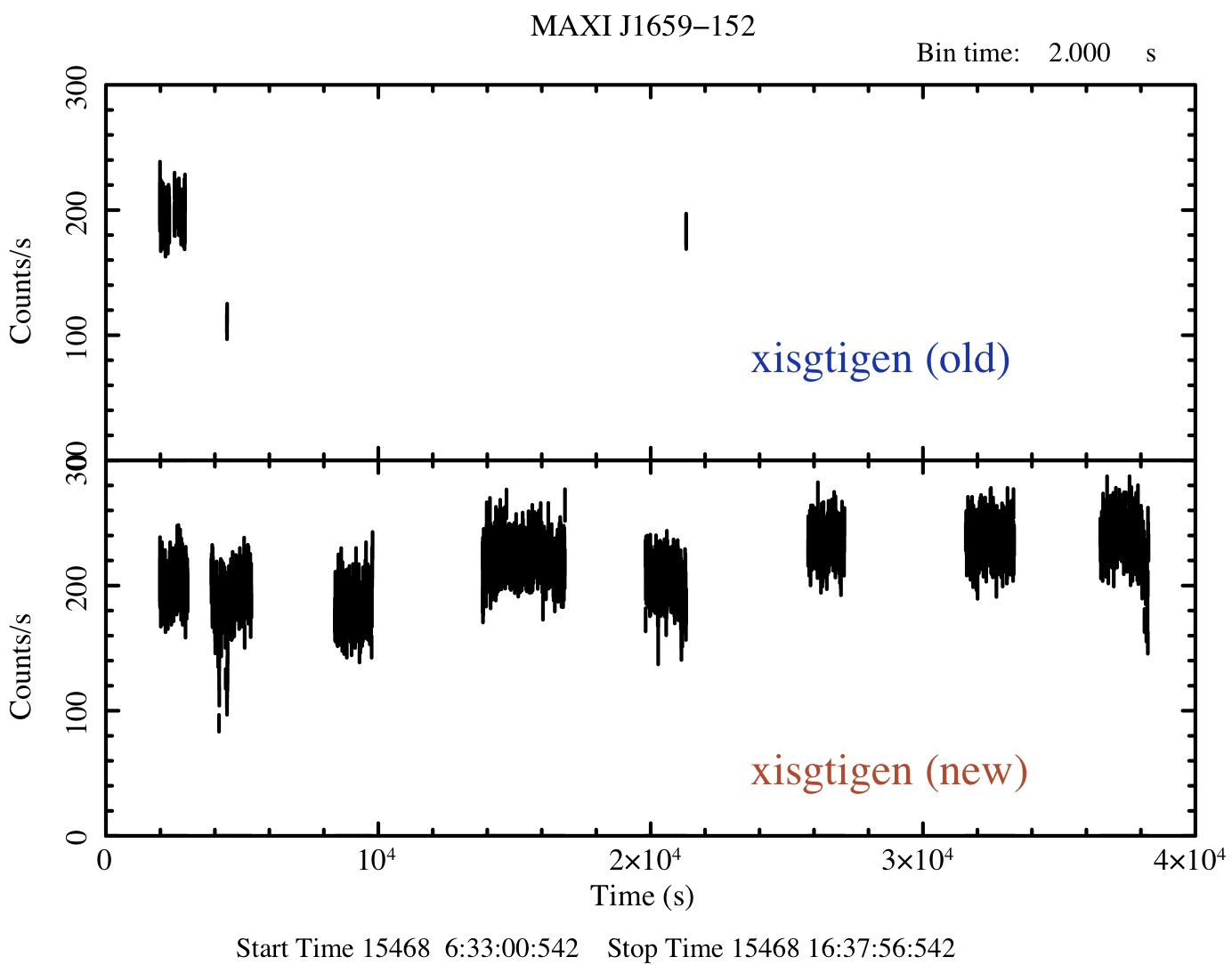
(top) The light curve of XIS0 taken from MAXIJ1659 filtered with gti files created from an old xisgtigen. (bottom) that filtered with the new xisgtigen.
Then we created two lightcurves. One is filtered with a gtifile created by an old xisgtigen, while the other with a new gtifile created by the new xisgitgen. You can see how the new xisgitgen works well to recover exposure time.
4 Examples
4.1 Case 1: Super Bright Source
Cyg X-1 is one of the persistent bright black hole binaries, so that pile-up effect cannot be avoidable even in its low/hard state, even if 1/4 window mode and burst option are utlized then.
This figure shows a result of aepileupcheckup.py, obtained from Cyg X-1 in the low/hard state taken on 2009 July 2. It tells us that the pile-up fraction becomes 3% at 59.9 pixels, and 1% at 97.7 pixels.
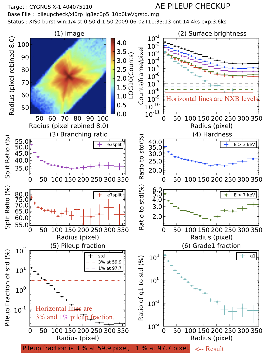
The output of aepileupcheckup.py in the case of Cyg X-1.
Te demonstrate how it worked, three spectra taken form the following three regions are compared,
- Region.1 (XIS*_whole.reg) -- a circle with a radius of 240 pixels from the source center.
- Region.2 (XIS*_pl3.reg) -- an annulus from a radius of 240 pixels to the radius of a pile-up fraction of 3% (59.9 pixels).
- Region.3 (XIS*_pl1.reg) -- an annulus from a radius of 240 pixels to the radius of a pile-up fraction of 1% (97.7 pixels).
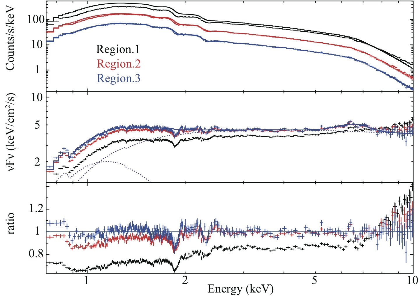
(top) Detector-response-convolved Cyg X-1 Spectra accumulated from the three regions. (middle) The same one as top, except for detector-response-removed ones. (bottom) The ratios of each spectra to the model of wabs(diskbb+powerlaw+gauss) fitted with the blue one (Region.3).
There region files are created by aepileupcheckup.py (see Step 2. Check Pileup Effects ). The three spectra created from the three regions are shown in figure. To clarify the spectral changes due to pileup, a comventional model is fitted to the spectra taken from Region 3, and the ratios to the model are also shown.
The one from Region.1 includes almost an entire CCD region, so it shows a decrease in low-energy flux by about 20% and a sharp increase in high-energy flux by 20%. In contrast, spectra taken from Region 2 and 3 are almost same, and thus pilueup effect is highly reduced. If you need more details, please check the Suzaku Pileup paper (Yamada et al. 2012) .
4.2 Case 2: Relaitvly Bright Source
MCG--6-30-15 is a typical Type I Seyfert galaxy, which has been actively studied in particular from ASCA era.
Its flux is as faint as about 5 m crab, and it is thought to be less affected by pile-up effect than Cyg X-1.
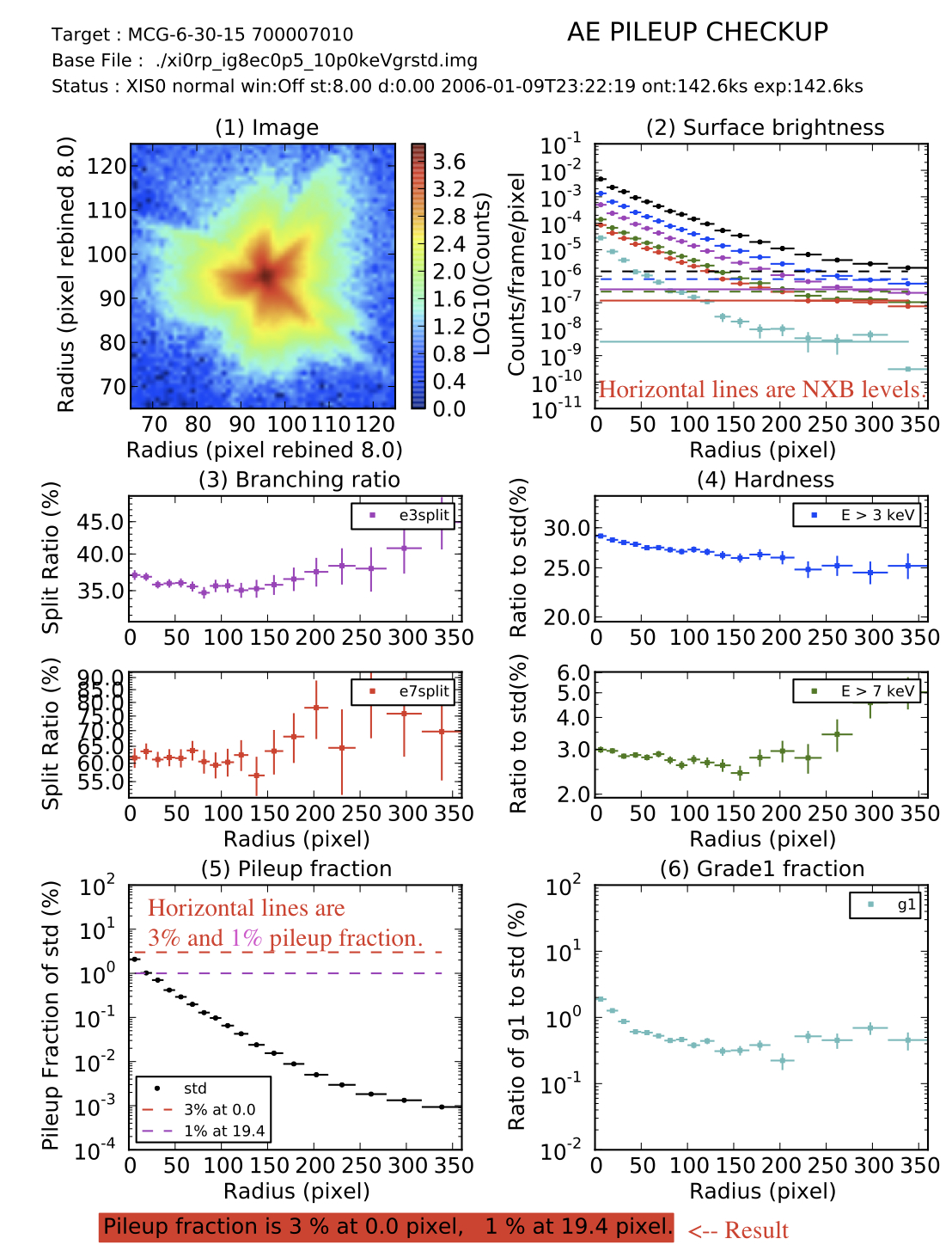
The output of aepileupcheckup.py in the case of MCG--6-30-15.
This figure shows a result of the aepileupcheck.py obtained from the XIS0 event of MCG--6-30-15 observed in 2006 January 9.
This tells us that the pile-up fraction of 3% becomes 0 pixel, and that of 1% at 19.4 pixel. Thus, the pile-up effect is thought to be almost negligible.
It should be noted that when the data is taken on a full window mode (a snap time of 8 s), a count rate integrated over the snap time could be relatively large enough to cause pileup effects.
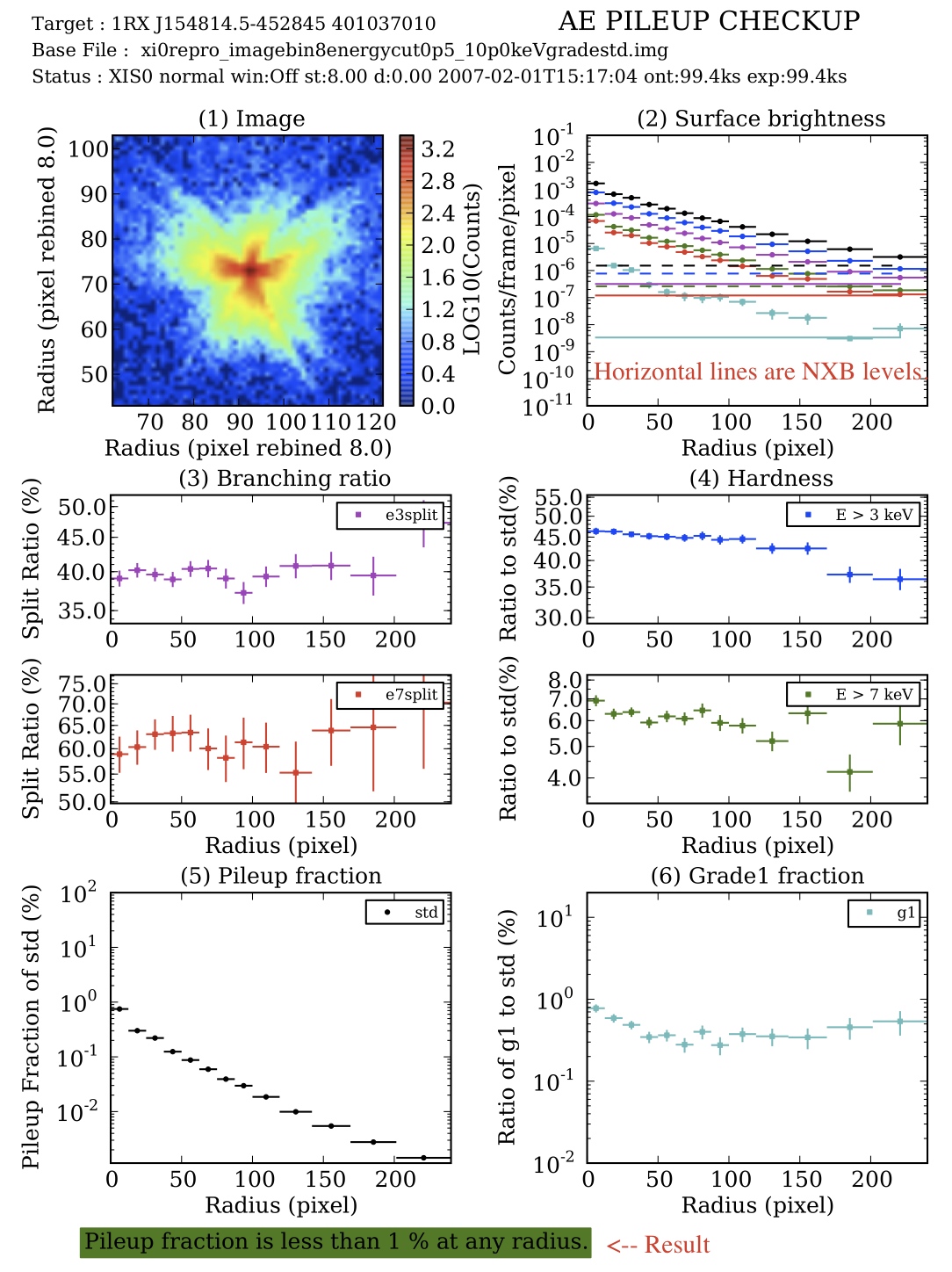
4.3 Case 3: Dimm Source
Finanly, the case free from pileup is shown with 1RX J154814.5-452845 taken on 2007 February 1 (401037010).
The results show that at any radius pilup fraction is less than 1%. When you see the same message, there is no worry about pileup.
The output of aeattitudetuned.py in the case of 1RX J154814.5-452845.
5 Details on softwares
5.1 Pileup Correction Tool : aepileupcheckup.py
This software reads WIN_SIZ from input fits keywords to approximately estimate the effetive area. In the case of HXD nominal position, the effective area is calucurated from the image itself, because an image at the position is asymetric at a large radius. This tool is also appilicable to P-sum mode.
The results consist of six parts and a resultant messasage.
- The XIS image created from standard event procesing. Make sure that your image is appropriate.
- The surface brightness of 0.5-10 keV standard event (black), 3-10 keV standard event (blue), 3-10 keV Grade2346 event (magenta), split event, 7-10 keV standard event (green), 7-10 keV Grade2346 event (red), and 0.5-10 keV Grade1 event (cyan). The horizontal lines are NXB levels derived from observation of NEP.
- The radial profile of Grade branching ratio in a unit of pixel: (top) E > 3 keV (bottom) E > 7 keV.
- The radial profile of hardness ratios in a unit of pixel : (top) E > 3 keV / 0.5-10 keV (bottom) E > 7 keV / 0.5-10 keV.
- The raidal profile of pileup fraction in a unit of pixel, together with 3% and 1% pileup fraction lines.
- The radial profile of the ratio of Grade 1 events to standard events in a unit of pixel.
When you need more help, please put the following command
> ./aepileupcheckup.py -h
The details on the method are summarized in the Suzaku Pileup paper (Yamada et al. 2012).
5.2 Attitude Correction Tool : aeattitudetuned.py
Here is an example of the usage when runing both attitude correction and cleansis:
> xis_extract_gradesortedimage.sh ver2/400003010 results/400003010/ONON ON ON
The first ON is to turn on aeattitudetunded.py, while the second ON is to turn on cleansis.
When you directly run aeattitudetunded.py, then please read the following.
You need to prepare the three files in your working directory.
- a cleaned event fits file
- an image fits file, rebinned as xybinsize 1
- an attitude file (included in auxil/ae*obsid*.att.gz )
We recommend that you input cleaned events not unscreened events, because the unscreened events include off-source events. The input image fits is needed for convertion of RA and DEC to SKYX and SKYY in kapteyn modules, and must be rebinned as putting set xybinsize 1 in extracging an image in xselect.
The input parameters for aeattitudetuned.py are inputfits imagefits input_attfile output_attfile. The figure is an exmple of aeattitudetunded.py when applying to ALGOL data. The command at that time is as follows:
> ./aeattitudetuned.py xi0_cleaned.evt xi0_rebin1.img new.att
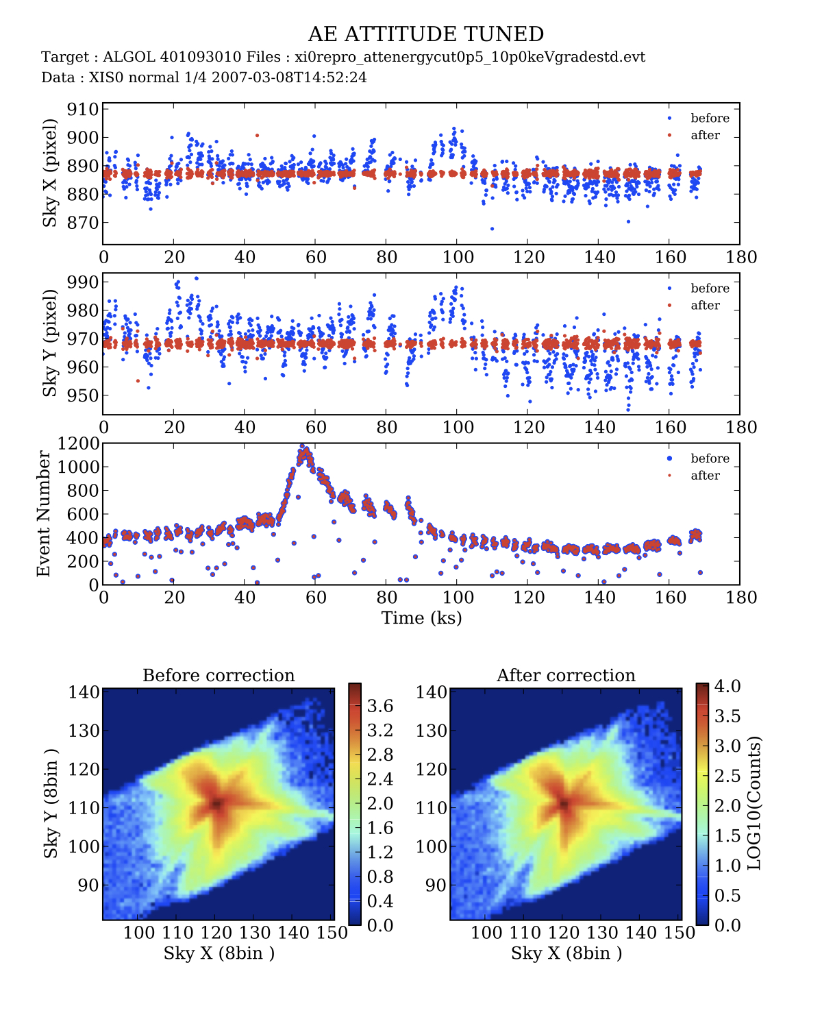
The output of aeattitudetuned.py in the case of ALGOL.
After creating a new attitude file, you must reprocess the XIS events by runing xiscoord with the new attitude file, and run xissimarfgen with the new attitude file.
The attitude correction is based on aeattcor.sl (http://space.mit.edu/CXC/software/suzaku/) created by M. Nowak and others.
When you need more help, please put the following command
> ./aeattitudetuned.py -h
6 History
- February, 2012 by S. Yamada et al. / ver 1.0 is created.
- Janurary, 2019 by S. Yamada / ver 2.0 is created not to use kapteyn.