


The final results of using XSPEC are usually one or more tables containing confidence ranges and fit statistics, and one or more plots showing the fits themselves. So far, all the plots shown have the default settings, but it is possible to edit plots to get closer to the appearance what you want.
The plotting package used by XSPEC is PGPLOT, which is comprised of a library of low-level tasks. At a higher level is QDP, the interactive program that forms the interface between the XSPEC user and PGPLOT. QDP has its own manual; it also comes with on-line help. Here, we show how to make some of the most common modifications to plots.
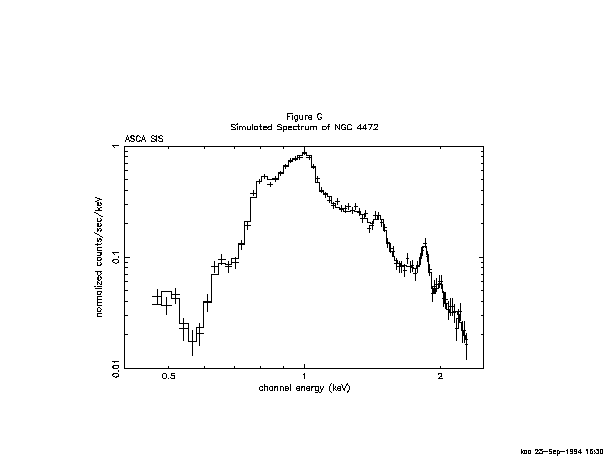
To initiate interactive plotting in XSPEC, use the command iplot instead of the usual plot. In this example, we'll take the simulated ASCA SIS spectrum of the previous section and make the following modifications to the data plot:
After the iplot command, the plot itself appears, followed by the QDP prompt:
 XSPEC> iplot data
 PLT>
The first thing we'll do is change the aspect ratio of the box that contains the plot (viewport in QDP terminology). The viewport is defined by the coordinates of the lower left and upper right corners of the page, normalized so that the width and height of the page are unity. The labels fall outside the viewport, so if the full viewport were specified, only the plot would appear. The default box has a viewport with corners at (0.1, 0.1) and (0.9, 0.9). For our purposes, we want a viewport with corners at (0.2, 0.2) and (0.8, 0.7): with this size and shape, the hardcopy will fit nicely on the page and not have to be reduced for photocopying. To change the viewport, use the command viewport followed by the coordinates:
PLT> viewport 0.2 0.2 0.8 0.7
Next we want to change two of the labels: the label at the top, which currently says only data, and the label that specifies the filename. This change is a straightforward one using the label command, which takes as arguments a location description and the text string:
 PLT> label top Simulated Spectrum of NGC 4472
 PLT> label file ASCA SIS
Other location descriptors are available, including x and y for the x-axis and y-axis, respectively. To get help on a QDP command, type help followed by the name of the command at the PLT> prompt. Note that QDP commands can be abbreviated, just like XSPEC commands. To see the results of changing the viewport and the labels, just enter the command plot:
PLT> plot
The two changes we want to make next are to rescale the axes and to change the y-axis to a logarithmic scale. The commands for these changes also are straightforward: the rescale command takes the minimum and maximum values as its arguments, while the log command takes x or y as arguments:
 PLT> rescale x 0.4 2.5
 PLT> rescale y 0.01 1
 PLT> log y
To revert to a linear scale, use the command log off y. All that is left to change are the thickness of the lines (the default, least for postscript files that are turned into hardcopies, is too fine) and the size of the characters (we want slightly smaller characters). The lwidth command does the former: it takes a width as its argument: the default is 1: we'll reset it to 3. The çsize command does the latter, taking a normalization as its argument. One (1) will not change the size, a number less than one will reduce it and a number bigger than one will increase it.
 PLT> lwidth 3
 PLT> csize 0.8
Finally, to produce a postscript file that we can print, we use the hardcopy command:
PLT> hardcopy ngc4472_sis.ps/ps
Here, we have given the file the name ngc4472_sis.ps. It will be written into the current directory. The suffix /ps tells the program to produce a postscript file.
The result of all this manipulation is shown proudly in Figure G.